Data Mining Techniques for Malware Detection R

Data Mining Techniques for Malware Detection R. K. Agrawal School of Computer and Systems Sciences Jawaharlal Nehru University New. Delhi-110067 1

Outline • Data Mining • Classification • Clustering • Association Rules • Experimental Results • Conclusion and Future Work 2

Motivation: “Necessity is the Mother of Invention • Data explosion problem – Automated data collection tools lead to tremendous amounts of data stored in databases and other information repositories • We are drowning in data, but starving for knowledge! • Solution: data mining – Extraction of interesting knowledge (rules, regularities, patterns, constraints) from data in large databases 3

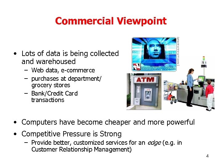Commercial Viewpoint • Lots of data is being collected and warehoused – Web data, e-commerce – purchases at department/ grocery stores – Bank/Credit Card transactions • Computers have become cheaper and more powerful • Competitive Pressure is Strong – Provide better, customized services for an edge (e. g. in Customer Relationship Management) 4

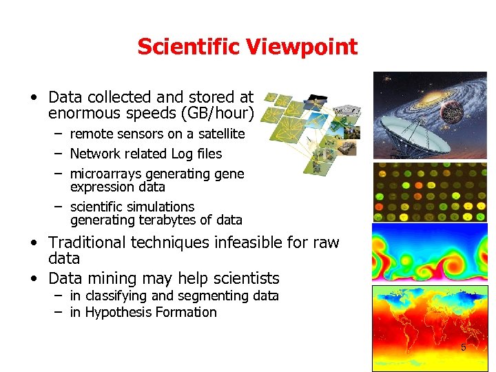Scientific Viewpoint • Data collected and stored at enormous speeds (GB/hour) – remote sensors on a satellite – Network related Log files – microarrays generating gene expression data – scientific simulations generating terabytes of data • Traditional techniques infeasible for raw data • Data mining may help scientists – in classifying and segmenting data – in Hypothesis Formation 5

What Is Data Mining? • Data mining (knowledge discovery in databases): – Extraction of interesting (non-trivial, implicit, previously unknown and potentially useful) information or patterns from data in large databases • Alternative names: – Knowledge discovery(mining) in databases (KDD), knowledge extraction, data/pattern analysis, data archeology, business intelligence, etc. 6

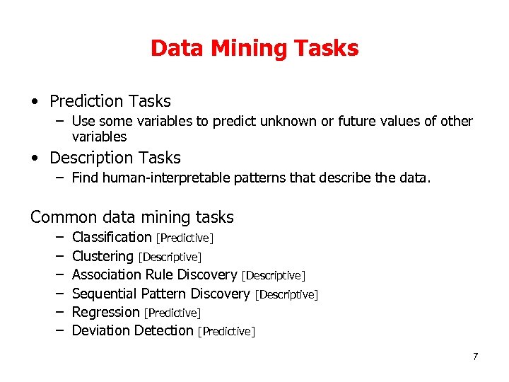Data Mining Tasks • Prediction Tasks – Use some variables to predict unknown or future values of other variables • Description Tasks – Find human-interpretable patterns that describe the data. Common data mining tasks – – – Classification [Predictive] Clustering [Descriptive] Association Rule Discovery [Descriptive] Sequential Pattern Discovery [Descriptive] Regression [Predictive] Deviation Detection [Predictive] 7

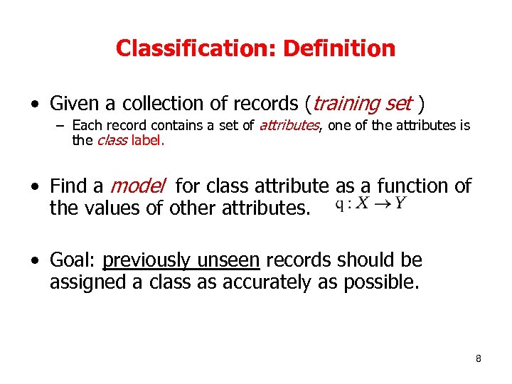Classification: Definition • Given a collection of records (training set ) – Each record contains a set of attributes, one of the attributes is the class label. • Find a model for class attribute as a function of the values of other attributes. • Goal: previously unseen records should be assigned a class as accurately as possible. 8

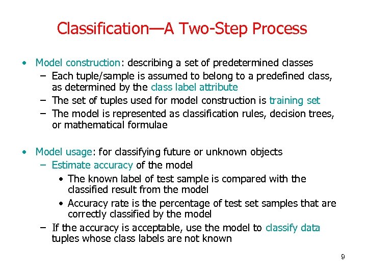Classification—A Two-Step Process • Model construction: describing a set of predetermined classes – Each tuple/sample is assumed to belong to a predefined class, as determined by the class label attribute – The set of tuples used for model construction is training set – The model is represented as classification rules, decision trees, or mathematical formulae • Model usage: for classifying future or unknown objects – Estimate accuracy of the model • The known label of test sample is compared with the classified result from the model • Accuracy rate is the percentage of test set samples that are correctly classified by the model – If the accuracy is acceptable, use the model to classify data tuples whose class labels are not known 9

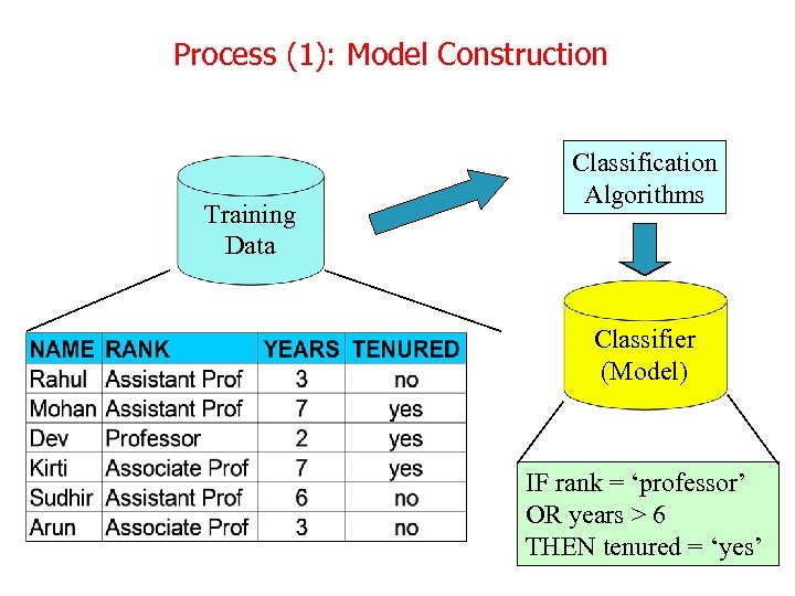Process (1): Model Construction Training Data Classification Algorithms Classifier (Model) IF rank = ‘professor’ OR years > 6 THEN tenured = ‘yes’ 10

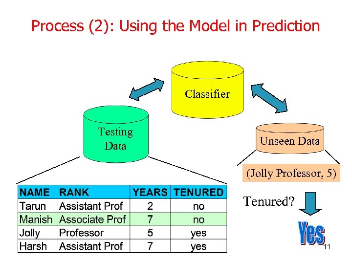Process (2): Using the Model in Prediction Classifier Testing Data Unseen Data (Jolly Professor, 5) Tenured? 11

Classification: Application • Malware Detection – Goal: Predict whether the given binary is Malware or not. – Approach: • Use both kind of binaries (Normal and Malware) • Learn a model for the class of the binaries. • Use this model to detect malware by observing a binary. 12

Clustering Definition • Given a set of data points, each having a set of attributes, and a similarity measure among them, find clusters such that – Data points in one cluster are more similar to one another. – Data points in separate clusters are less similar to one another. • Similarity Measures: – Euclidean Distance if attributes are continuous. – Other Problem-specific Measures. 13

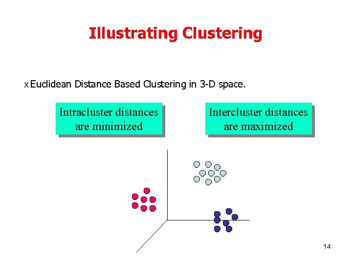Illustrating Clustering x Euclidean Distance Based Clustering in 3 -D space. Intracluster distances are minimized Intercluster distances are maximized 14

Clustering: Application • Binaries Segmentation: – Goal: subdivide a given set of binaries into distinct subsets of binaries 15

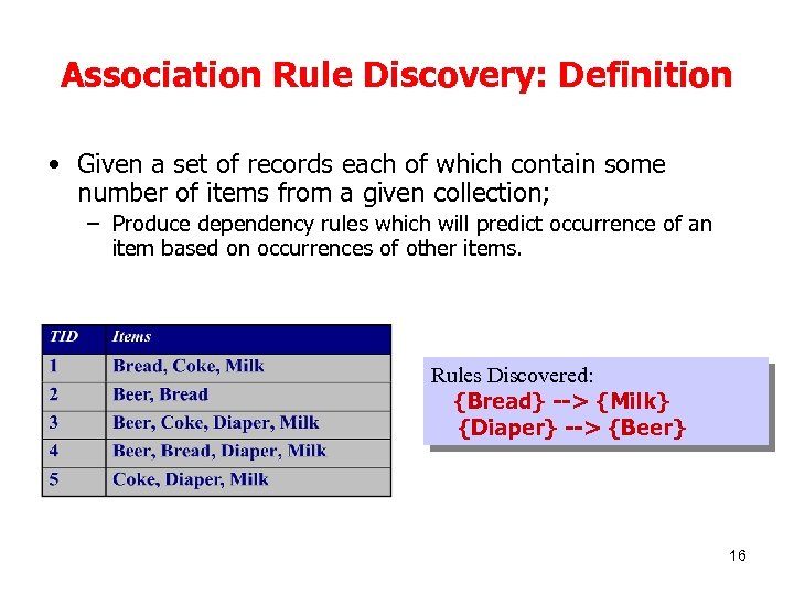Association Rule Discovery: Definition • Given a set of records each of which contain some number of items from a given collection; – Produce dependency rules which will predict occurrence of an item based on occurrences of other items. Rules Discovered: {Bread} --> {Milk} {Diaper} --> {Beer} 16

The Sad Truth About Diapers and Beer • So, don’t be surprised if you find six-packs stacked next to diapers! 17

Association Rule Discovery: Application • Malware Rules – Goal: To identify activities that are happen together in a given malware. 18

Sequential Pattern Discovery: Definition Given is a set of objects, with each object associated with its own timeline of events, find rules that predict strong sequential dependencies among different events: – In telecommunications alarm logs, • (Inverter_Problem Excessive_Line_Current) (Rectifier_Alarm) --> (Fire_Alarm) – In point-of-sale transaction sequences, • Computer Bookstore: (Intro_To_Visual_C) (C++_Primer) --> (Perl_for_dummies) • Athletic Apparel Store: (Shoes) (Racket, Racketball) --> (Sports_Jacket) 19

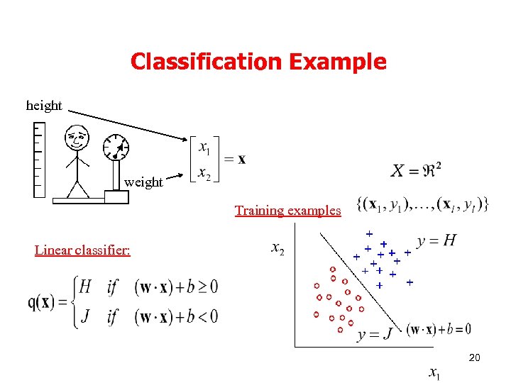Classification Example height weight Training examples Linear classifier: 20

Classification Techniques • • • Decision Trees Naïve Bayes Support Vector Machines Neural Networks Parzen Window K-nearest neigbor 21

Issues: Data Preparation • Data cleaning – Preprocess data in order to reduce noise and handle missing values • Relevance analysis (feature selection) – Remove the irrelevant or redundant attributes • Data transformation – Generalize and/or normalize data 22

Issues: Evaluating Classification Methods • Accuracy – classifier accuracy: predicting class label – predictor accuracy: guessing value of predicted attributes • Speed – time to construct the model (training time) – time to use the model (classification/prediction time) • Robustness: handling noise and missing values • Scalability: efficiency in disk-resident databases • Interpretability – understanding and insight provided by the model • Other measures, e. g. , goodness of rules, such as decision tree size or compactness of classification rules 23

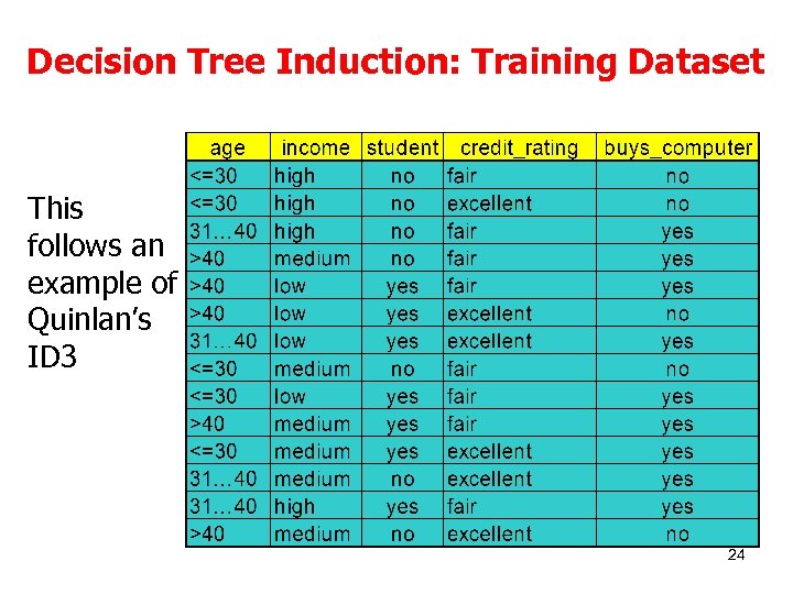Decision Tree Induction: Training Dataset This follows an example of Quinlan’s ID 3 24

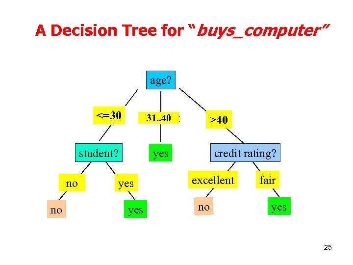A Decision Tree for “buys_computer” age? <=30 31. . 40 overcast student? no no >40 credit rating? yes yes excellent no fair yes 25

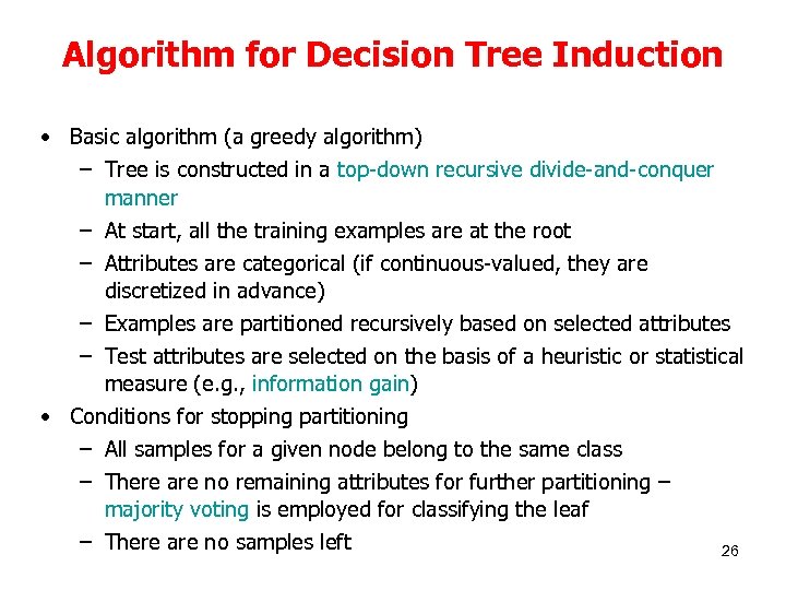Algorithm for Decision Tree Induction • Basic algorithm (a greedy algorithm) – Tree is constructed in a top-down recursive divide-and-conquer manner – At start, all the training examples are at the root – Attributes are categorical (if continuous-valued, they are discretized in advance) – Examples are partitioned recursively based on selected attributes – Test attributes are selected on the basis of a heuristic or statistical measure (e. g. , information gain) • Conditions for stopping partitioning – All samples for a given node belong to the same class – There are no remaining attributes for further partitioning – majority voting is employed for classifying the leaf – There are no samples left 26

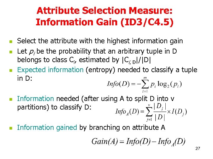Attribute Selection Measure: Information Gain (ID 3/C 4. 5) n n n Select the attribute with the highest information gain Let pi be the probability that an arbitrary tuple in D belongs to class Ci, estimated by |Ci, D|/|D| Expected information (entropy) needed to classify a tuple in D: Information needed (after using A to split D into v partitions) to classify D: Information gained by branching on attribute A 27

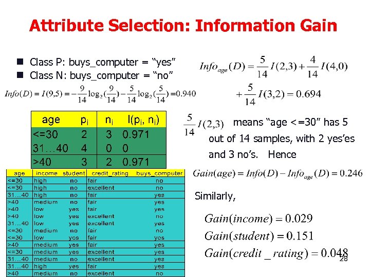Attribute Selection: Information Gain Class P: buys_computer = “yes” g Class N: buys_computer = “no” g means “age <=30” has 5 out of 14 samples, with 2 yes’es and 3 no’s. Hence Similarly, 28

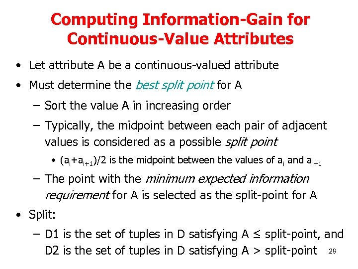Computing Information-Gain for Continuous-Value Attributes • Let attribute A be a continuous-valued attribute • Must determine the best split point for A – Sort the value A in increasing order – Typically, the midpoint between each pair of adjacent values is considered as a possible split point • (ai+ai+1)/2 is the midpoint between the values of ai and ai+1 – The point with the minimum expected information requirement for A is selected as the split-point for A • Split: – D 1 is the set of tuples in D satisfying A ≤ split-point, and D 2 is the set of tuples in D satisfying A > split-point 29

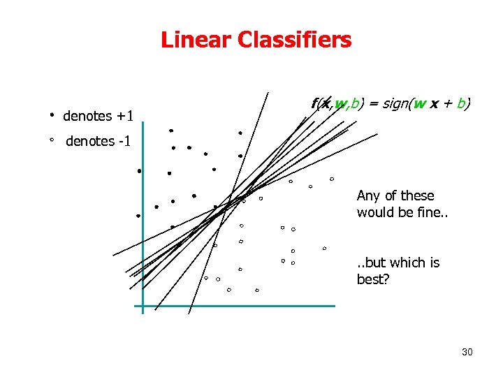Linear Classifiers denotes +1 f(x, w, b) = sign(w x + b) denotes -1 Any of these would be fine. . but which is best? 30

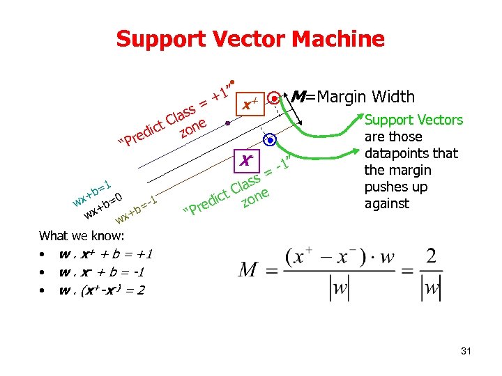Support Vector Machine 1” + = + x s las e C ict zon d Pre “ 1 b= 0 + = -1 wx +b b= + wx wx X- M=Margin Width -1” = “P ss la t C one c z edi r Support Vectors are those datapoints that the margin pushes up against What we know: • w. x+ + b = +1 • w. x- + b = -1 • w. (x+-x-) = 2 31

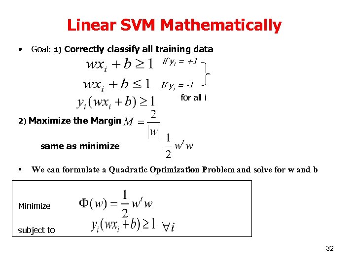Linear SVM Mathematically • Goal: 1) Correctly classify all training data if yi = +1 If yi = -1 for all i 2) Maximize the Margin same as minimize • We can formulate a Quadratic Optimization Problem and solve for w and b Minimize subject to 32

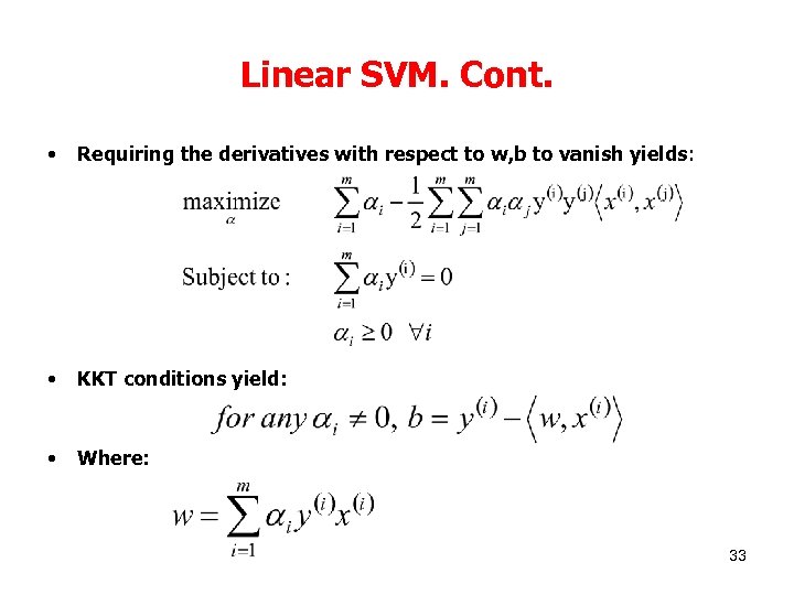Linear SVM. Cont. • Requiring the derivatives with respect to w, b to vanish yields: • KKT conditions yield: • Where: 33

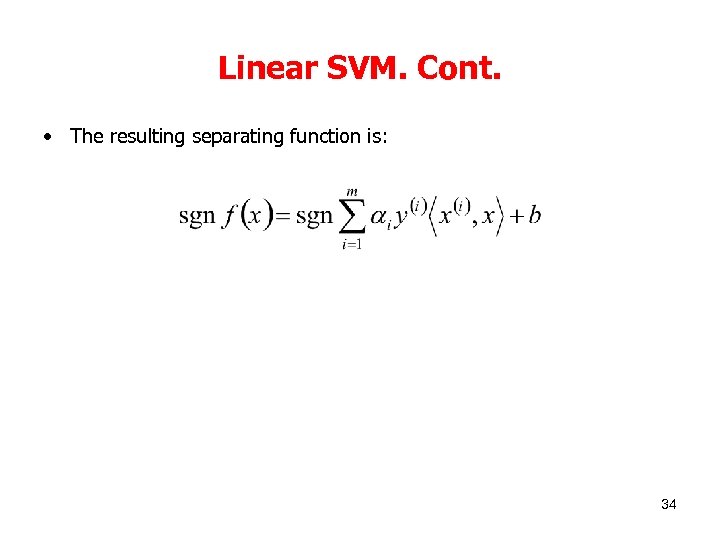Linear SVM. Cont. • The resulting separating function is: 34

Linear SVM. Cont. • Requiring the derivatives with respect to w, b to vanish yields: • KKT conditions yield: • Where: 35

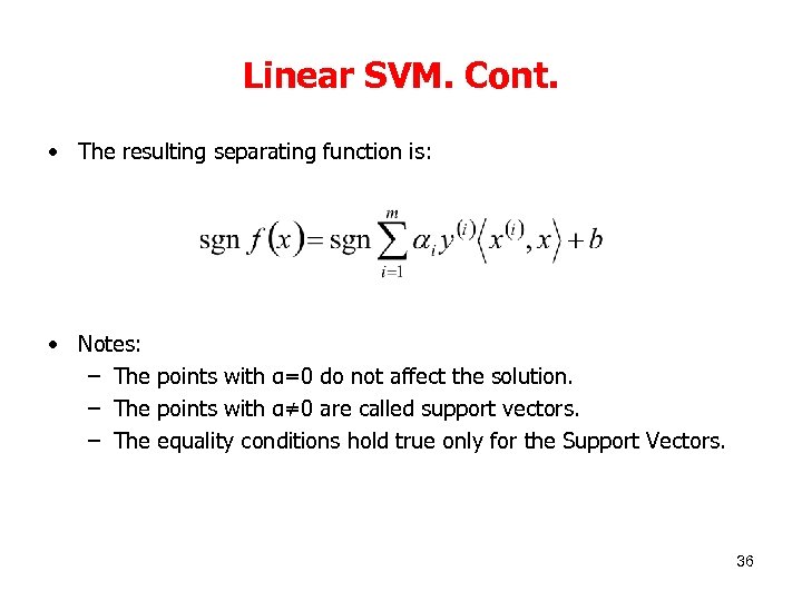Linear SVM. Cont. • The resulting separating function is: • Notes: – The points with α=0 do not affect the solution. – The points with α≠ 0 are called support vectors. – The equality conditions hold true only for the Support Vectors. 36

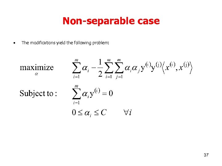Non-separable case • The modifications yield the following problem: 37

Non Linear SVM • Note that the training data appears in the solution only in inner products. • If we pre-map the data into a higher and sparser space we can get more separability and a stronger separation family of functions. • The pre-mapping might make the problem infeasible. • We want to avoid pre-mapping and still have the same separation ability. • Suppose we have a simple function that operates on two training points and implements an inner product of their pre-mappings, then we achieve better separation with no added cost. 38

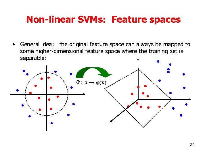Non-linear SVMs: Feature spaces • General idea: the original feature space can always be mapped to some higher-dimensional feature space where the training set is separable: Φ: x → φ(x) 39

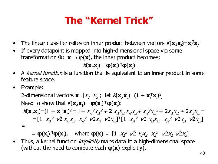The “Kernel Trick” • • • The linear classifier relies on inner product between vectors K(xi, xj)=xi. Txj If every datapoint is mapped into high-dimensional space via some transformation Φ: x → φ(x), the inner product becomes: K(xi, xj)= φ(xi) Tφ(xj) A kernel function is a function that is equivalent to an inner product in some feature space. Example: 2 -dimensional vectors x=[x 1 x 2]; let K(xi, xj)=(1 + xi. Txj)2, Need to show that K(xi, xj)= φ(xi) Tφ(xj): K(xi, xj)=(1 + xi. Txj)2, = 1+ xi 12 xj 12 + 2 xi 1 xj 1 xi 2 xj 2+ xi 22 xj 22 + 2 xi 1 xj 1 + 2 xi 2 xj 2= = [1 xi 12 √ 2 xi 1 xi 22 √ 2 xi 1 √ 2 xi 2]T [1 xj 12 √ 2 xj 1 xj 22 √ 2 xj 1 √ 2 xj 2] = = φ(xi) Tφ(xj), where φ(x) = [1 x 12 √ 2 x 1 x 2 x 22 √ 2 x 1 √ 2 x 2] Thus, a kernel function implicitly maps data to a high-dimensional space (without the need to compute each φ(x) explicitly). 40

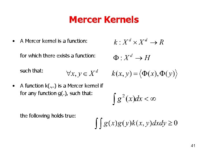Mercer Kernels • A Mercer kernel is a function: for which there exists a function: such that: • A function k(. , . ) is a Mercer kernel if for any function g(. ), such that: the following holds true: 41

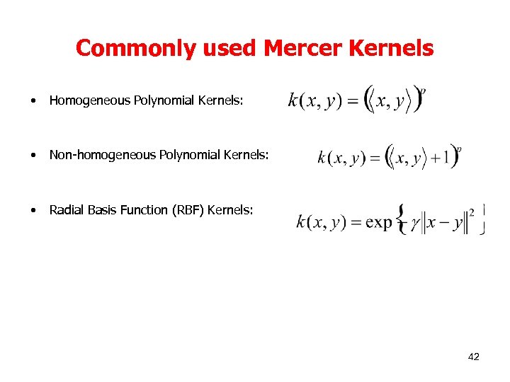Commonly used Mercer Kernels • Homogeneous Polynomial Kernels: • Non-homogeneous Polynomial Kernels: • Radial Basis Function (RBF) Kernels: 42

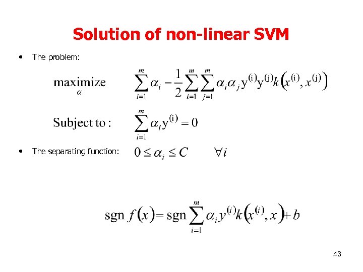Solution of non-linear SVM • The problem: • The separating function: 43

Multi-Class SVM • Approaches: • One against One ( K (K-1) / 2 ) binary Classifiers required Outputs of the classifiers are aggregated to make the final decision. • One against All (K binary Classifiers required): It trains k binary classifiers, each of which separates one class from the other (k-1) classes. Given a data point X , the binary classifier with the largest output determines the class of X. 44

Why Is SVM Effective on High Dimensional Data? n The complexity of trained classifier is characterized by the # of support vectors rather than the dimensionality of the data n The support vectors are the essential or critical training examples — they lie closest to the decision boundary (MMH) n If all other training examples are removed and the training is repeated, the same separating hyperplane would be found n The number of support vectors found can be used to compute an (upper) bound on the expected error rate of the SVM classifier, which is independent of the data dimensionality n Thus, an SVM with a small number of support vectors can have good generalization, even when the dimensionality of the data is high 45

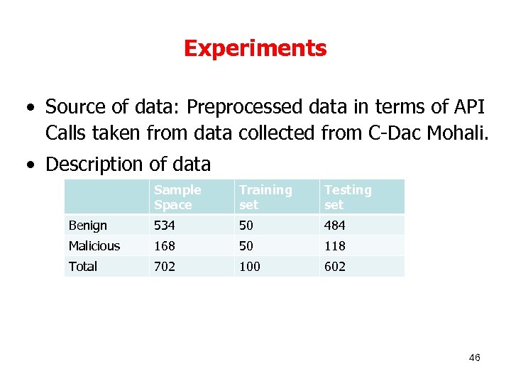Experiments • Source of data: Preprocessed data in terms of API Calls taken from data collected from C-Dac Mohali. • Description of data Sample Space Training set Testing set Benign 534 50 484 Malicious 168 50 118 Total 702 100 602 46

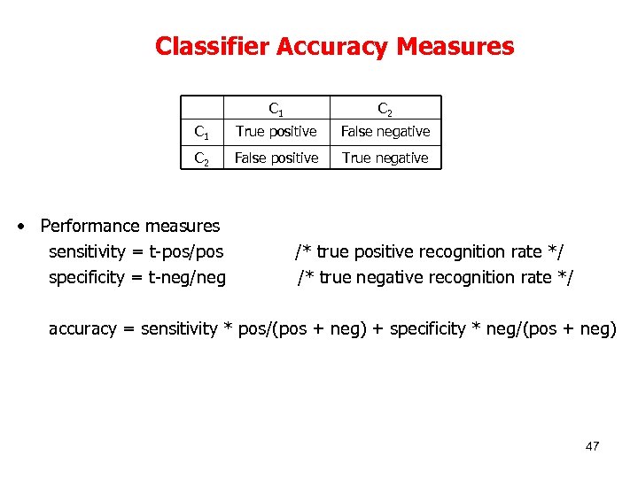Classifier Accuracy Measures C 1 C 2 C 1 True positive False negative C 2 False positive True negative • Performance measures sensitivity = t-pos/pos /* true positive recognition rate */ specificity = t-neg/neg /* true negative recognition rate */ accuracy = sensitivity * pos/(pos + neg) + specificity * neg/(pos + neg) 47

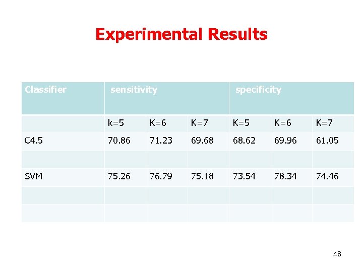Experimental Results Classifier sensitivity specificity k=5 K=6 K=7 K=5 K=6 K=7 C 4. 5 70. 86 71. 23 69. 68 68. 62 69. 96 61. 05 SVM 75. 26 76. 79 75. 18 73. 54 78. 34 74. 46 48

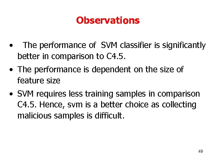Observations • The performance of SVM classifier is significantly better in comparison to C 4. 5. • The performance is dependent on the size of feature size • SVM requires less training samples in comparison C 4. 5. Hence, svm is a better choice as collecting malicious samples is difficult. 49

Conclusion & Future Work • SVM is a better classification technique which can be used for detection of Malware. • Needs attention to construct better feature representation for better generalization • How to extend it to multi-class malware problem 50

References • C. J. C. Burges. A Tutorial on Support Vector Machines for Pattern Recognition. Data Mining and Knowledge Discovery, 2(2): 121 -168, 1998. • J. R. Quinlan. C 4. 5: Programs for Machine Learning. Morgan Kaufmann, 1993. • P. Tan, M. Steinbach, and V. Kumar. Introduction to Data Mining. Addison Wesley, 2005. • I. H. Witten and E. Frank. Data Mining: Practical Machine Learning Tools and Techniques, 2 ed. Morgan Kaufmann, 2005. • • Han and Kamber, Data Mining Concepts B. Zhang, J. Yin, J. Hao, D. Zhang, S. Wang, Using Support Vector Machine to detect unknown computer viruses, Int. Journal of Computational Intelligence Research, vol. 2, No. 1, pp. 100 -104, 2006. Szappanos, G. : Are There Any Polymorphic Macro Viruses at ALL (and What to Do with Them). in Proceedings of the 12 th International Virus Bulletin Conference, 2001. Forrest, S. , Hofmeyr, S. A. , Somayaji, A. : Computer immunology. Communications of the ACM. 10, pp. 88– 96, 1997. Lee, W. , Dong, X. : Information-Theoretic measures for anomaly detection. In: Needham, R. , Abadi M, (eds): . Proceedings of the 2001 IEEE Symposium on Security and Privacy Oakland, CA: IEEE Computer Society Press, pp. 130 -143, 2001. 51 LIBSVM. http: //www. csie. ntu. edu. tw/~cjlin/. • •

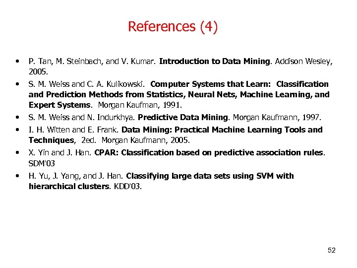References (4) • P. Tan, M. Steinbach, and V. Kumar. Introduction to Data Mining. Addison Wesley, 2005. • S. M. Weiss and C. A. Kulikowski. Computer Systems that Learn: Classification and Prediction Methods from Statistics, Neural Nets, Machine Learning, and Expert Systems. Morgan Kaufman, 1991. • S. M. Weiss and N. Indurkhya. Predictive Data Mining. Morgan Kaufmann, 1997. • I. H. Witten and E. Frank. Data Mining: Practical Machine Learning Tools and Techniques, 2 ed. Morgan Kaufmann, 2005. • X. Yin and J. Han. CPAR: Classification based on predictive association rules. SDM'03 • H. Yu, J. Yang, and J. Han. Classifying large data sets using SVM with hierarchical clusters. KDD'03. 52