Data Mining Techniques Classification Classification What

Data Mining Techniques: Classification

Classification • What is Classification? – Classifying tuples in a database – In training set E • each tuple consists of the same set of multiple attributes as the tuples in the large database W • additionally, each tuple has a known class identity – Derive the classification mechanism from the training set E, and then use this mechanism to classify general data (in W)

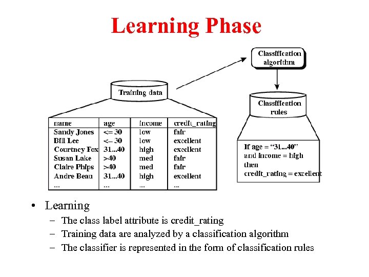Learning Phase • Learning – The class label attribute is credit_rating – Training data are analyzed by a classification algorithm – The classifier is represented in the form of classification rules

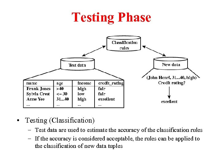Testing Phase • Testing (Classification) – Test data are used to estimate the accuracy of the classification rules – If the accuracy is considered acceptable, the rules can be applied to the classification of new data tuples

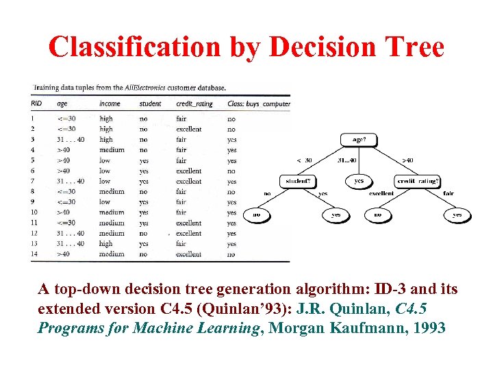Classification by Decision Tree A top-down decision tree generation algorithm: ID-3 and its extended version C 4. 5 (Quinlan’ 93): J. R. Quinlan, C 4. 5 Programs for Machine Learning, Morgan Kaufmann, 1993

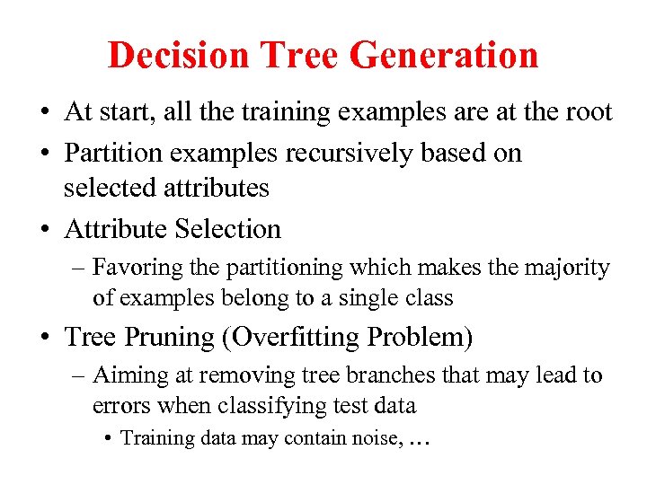Decision Tree Generation • At start, all the training examples are at the root • Partition examples recursively based on selected attributes • Attribute Selection – Favoring the partitioning which makes the majority of examples belong to a single class • Tree Pruning (Overfitting Problem) – Aiming at removing tree branches that may lead to errors when classifying test data • Training data may contain noise, …

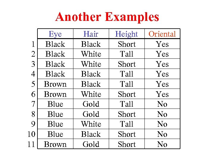Another Examples 1 2 3 4 5 6 7 8 9 10 11 Eye Black Brown Blue Brown Hair Black White Gold White Black Gold Height Short Tall Short Tall Short Oriental Yes Yes Yes No No No

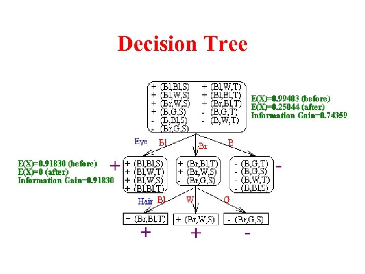Decision Tree

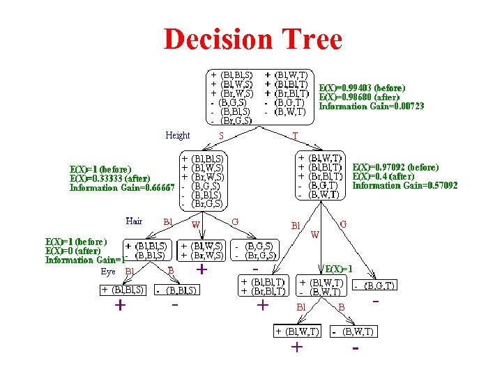Decision Tree

Decision Tree Generation • Attribute Selection (Split Criterion) – Information Gain (ID 3/C 4. 5/See 5) – Gini Index (CART/IBM Intelligent Miner) – Inference Power • These measures are also called goodness functions and used to select the attribute to split at a tree node during the tree generation phase

Decision Tree Generation • Branching Scheme – Determining the tree branch to which a sample belongs – Binary vs. K-ary Splitting • When to stop the further splitting of a node – Impurity Measure • Labeling Rule – A node is labeled as the class to which most samples at the node belongs

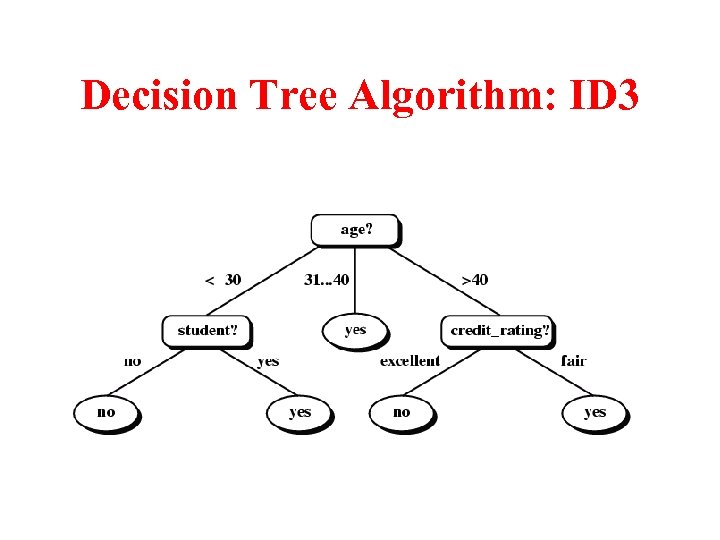
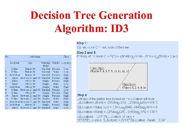
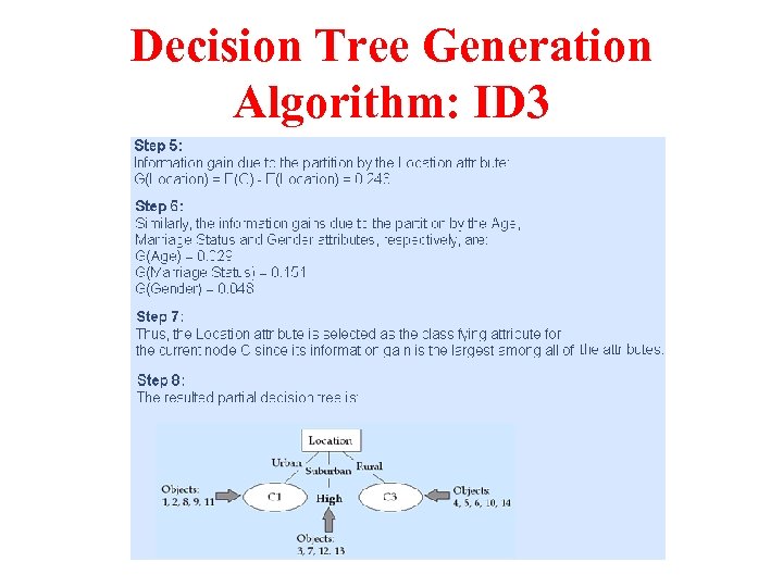
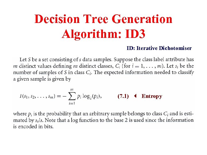Decision Tree Generation Algorithm: ID 3 ID: Iterative Dichotomiser (7. 1) Entropy

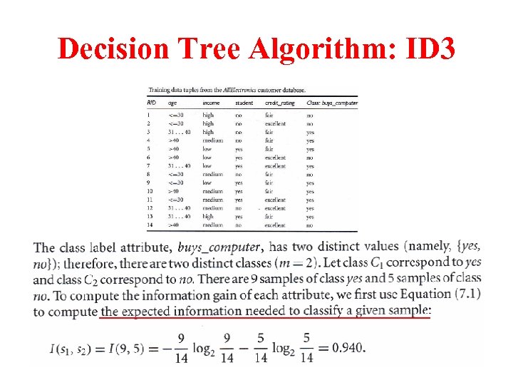Decision Tree Algorithm: ID 3

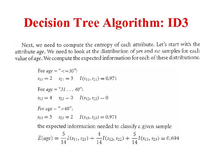Decision Tree Algorithm: ID 3

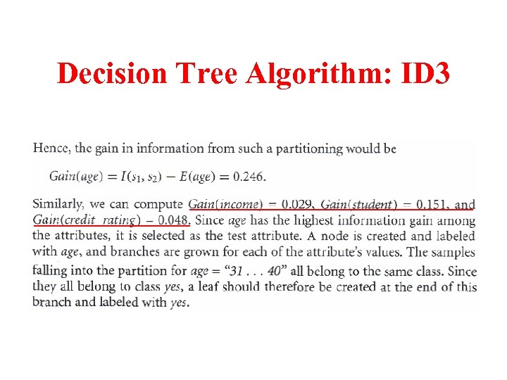Decision Tree Algorithm: ID 3

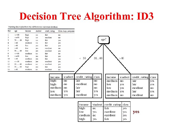Decision Tree Algorithm: ID 3 yes

Decision Tree Algorithm: ID 3

Exercise 2

Decision Tree Generation Algorithm: ID 3

Decision Tree Generation Algorithm: ID 3

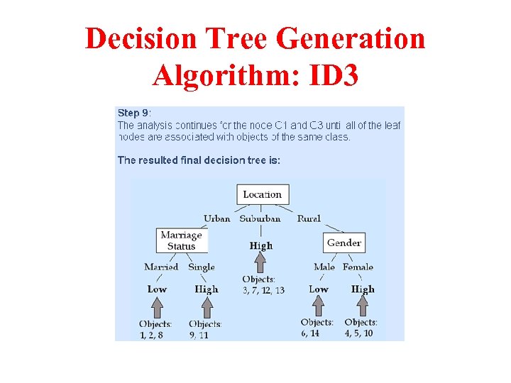Decision Tree Generation Algorithm: ID 3

How to Use a Tree • Directly – Test the attribute value of unknown sample against the tree. – A path is traced from root to a leaf which holds the label • Indirectly – Decision tree is converted to classification rules – One rule is created for each path from the root to a leaf – IF-THEN is easier for humans to understand

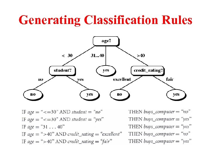Generating Classification Rules

Generating Classification Rules

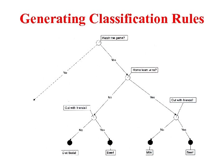
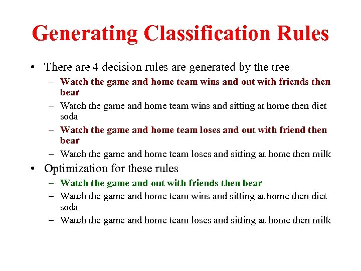Generating Classification Rules • There are 4 decision rules are generated by the tree – Watch the game and home team wins and out with friends then bear – Watch the game and home team wins and sitting at home then diet soda – Watch the game and home team loses and out with friend then bear – Watch the game and home team loses and sitting at home then milk • Optimization for these rules – Watch the game and out with friends then bear – Watch the game and home team wins and sitting at home then diet soda – Watch the game and home team loses and sitting at home then milk

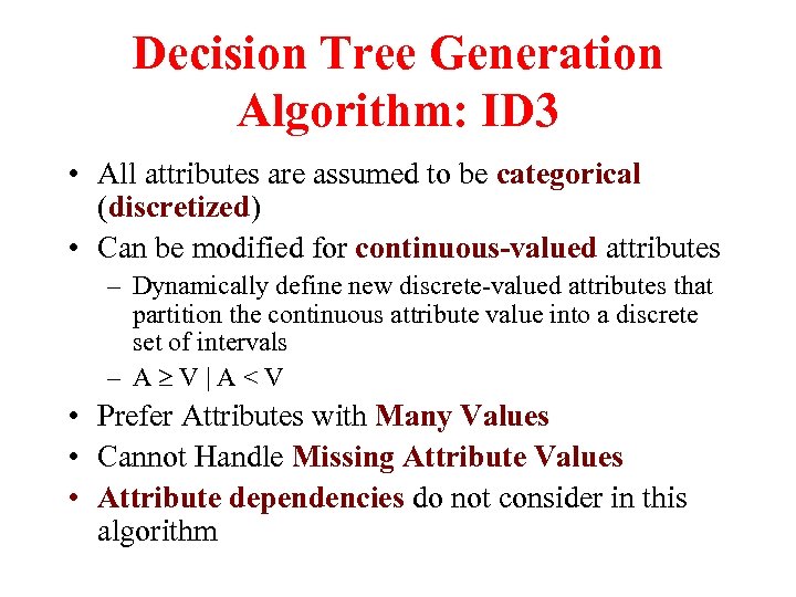Decision Tree Generation Algorithm: ID 3 • All attributes are assumed to be categorical (discretized) • Can be modified for continuous-valued attributes – Dynamically define new discrete-valued attributes that partition the continuous attribute value into a discrete set of intervals – A V|A

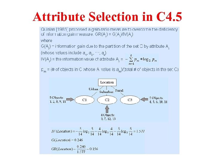Attribute Selection in C 4. 5

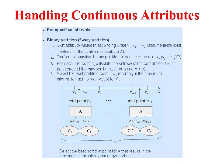Handling Continuous Attributes

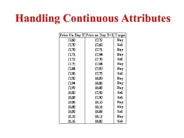Handling Continuous Attributes

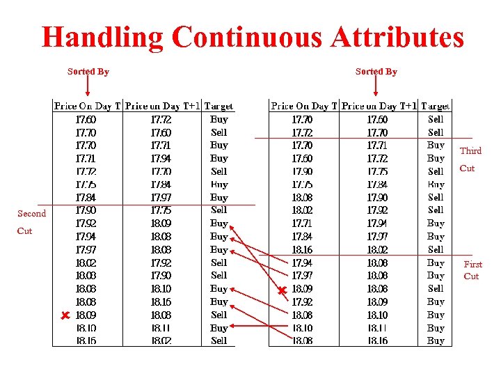Handling Continuous Attributes Sorted By Third Cut Second Cut First Cut

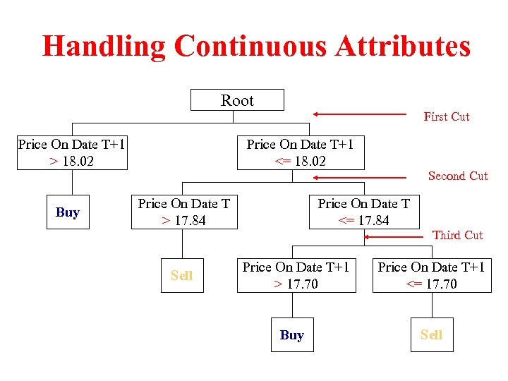Handling Continuous Attributes Root Price On Date T+1 > 18. 02 Buy First Cut Price On Date T+1 <= 18. 02 Price On Date T > 17. 84 Sell Second Cut Price On Date T <= 17. 84 Third Cut Price On Date T+1 > 17. 70 Price On Date T+1 <= 17. 70 Buy Sell

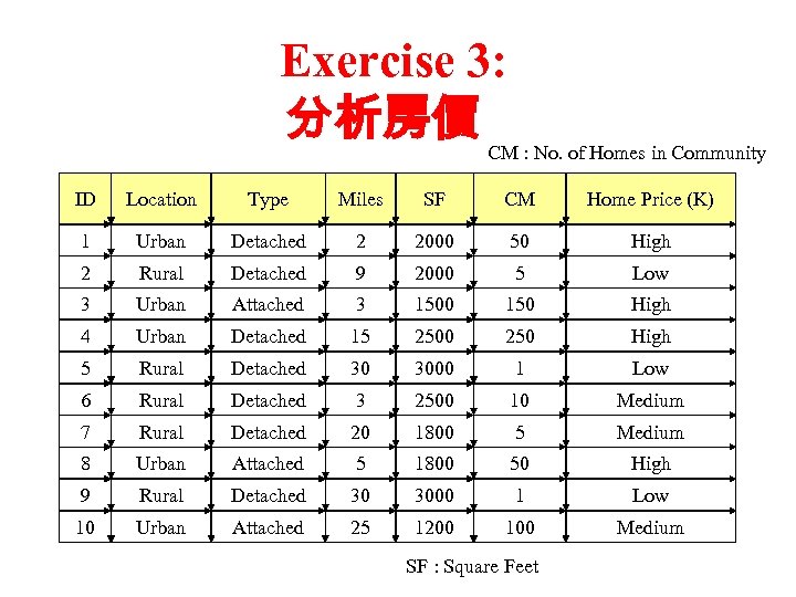Exercise 3: 分析房價 CM : No. of Homes in Community ID Location Type Miles SF CM Home Price (K) 1 Urban Detached 2 2000 50 High 2 Rural Detached 9 2000 5 Low 3 Urban Attached 3 1500 150 High 4 Urban Detached 15 2500 250 High 5 Rural Detached 30 3000 1 Low 6 Rural Detached 3 2500 10 Medium 7 Rural Detached 20 1800 5 Medium 8 Urban Attached 5 1800 50 High 9 Rural Detached 30 3000 1 Low 10 Urban Attached 25 1200 100 Medium SF : Square Feet

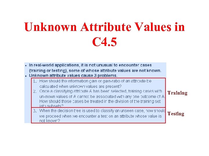Unknown Attribute Values in C 4. 5 Training Testing

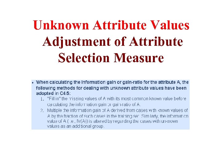Unknown Attribute Values Adjustment of Attribute Selection Measure

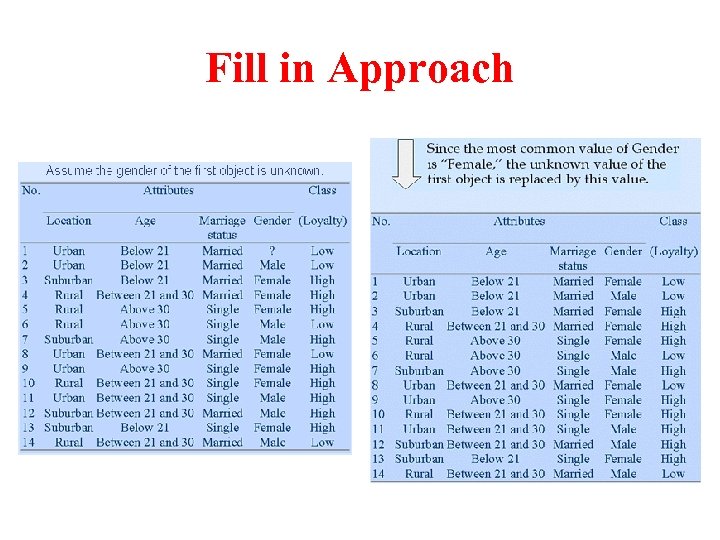Fill in Approach

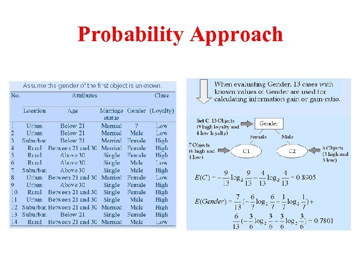Probability Approach

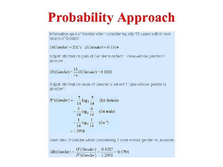Probability Approach

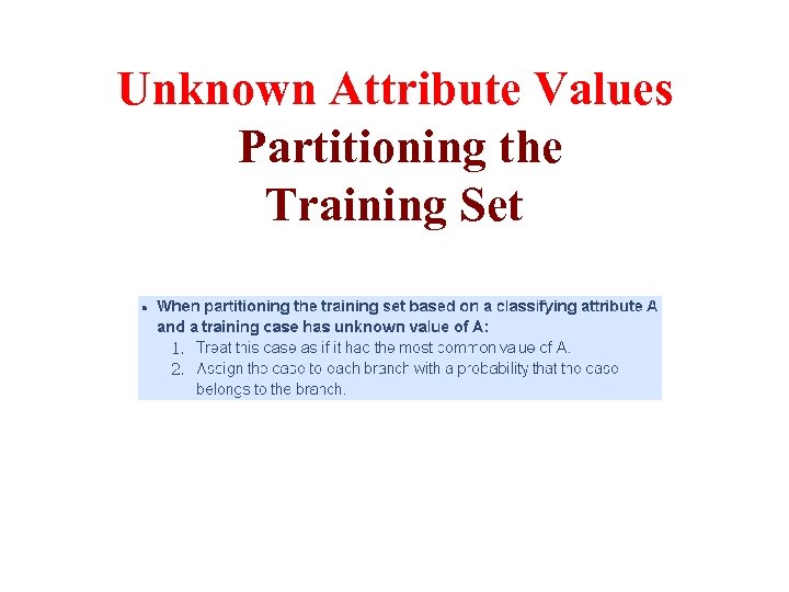Unknown Attribute Values Partitioning the Training Set

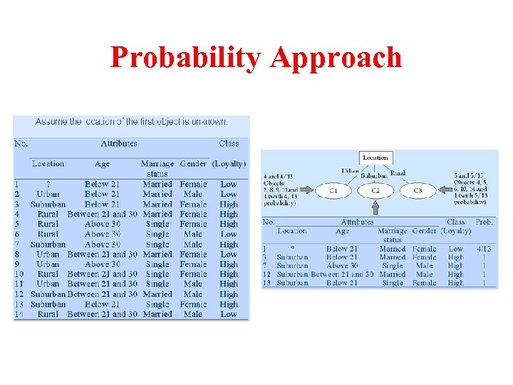Probability Approach

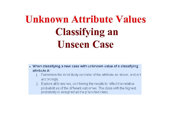Unknown Attribute Values Classifying an Unseen Case

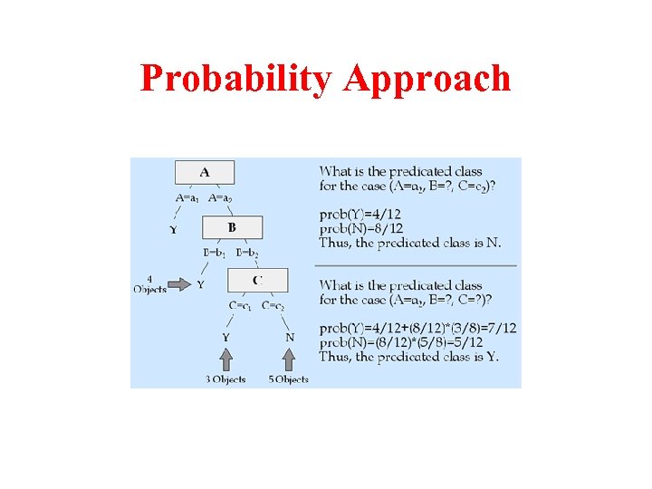Probability Approach

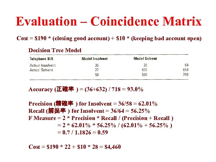Evaluation – Coincidence Matrix Cost = $190 * (closing good account) + $10 * (keeping bad account open) Decision Tree Model Accuracy (正確率 ) = (36+632) / 718 = 93. 0% Precision (精確率 ) for Insolvent = 36/58 = 62. 01% Recall (捕捉率 ) for Insolvent = 36/64 = 56. 25% F Measure = 2 * Precision * Recall / (Precision + Recall ) = 2 * 62. 01% * 56. 25% / (62. 01% + 56. 25% ) = 0. 7 / 1. 1826 = 0. 59 Cost = $190 * 22 + $10 * 28 = $4, 460

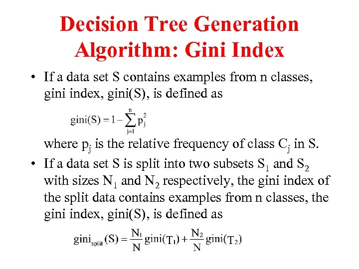Decision Tree Generation Algorithm: Gini Index • If a data set S contains examples from n classes, gini index, gini(S), is defined as where pj is the relative frequency of class Cj in S. • If a data set S is split into two subsets S 1 and S 2 with sizes N 1 and N 2 respectively, the gini index of the split data contains examples from n classes, the gini index, gini(S), is defined as

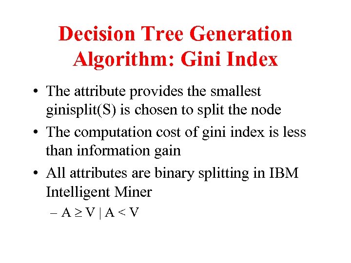Decision Tree Generation Algorithm: Gini Index • The attribute provides the smallest ginisplit(S) is chosen to split the node • The computation cost of gini index is less than information gain • All attributes are binary splitting in IBM Intelligent Miner –A V|A

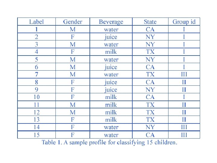
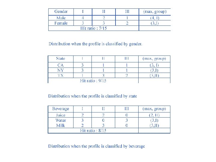
Decision Tree Generation Algorithm: Inference Power • A feature that is useful in inferring the group identity of a data tuple is said to have a good inference power to that group identity. • In Table 1, given attributes (features) “Gender”, “Beverage”, “State”, try to find their inference power to “Group id”

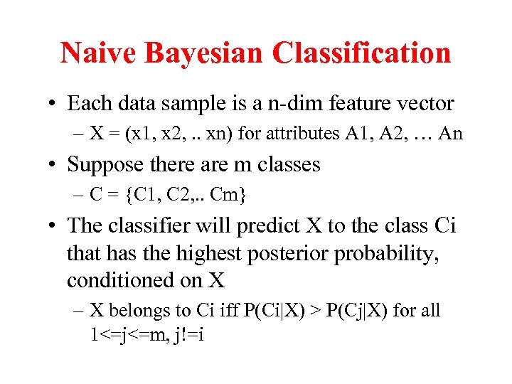Naive Bayesian Classification • Each data sample is a n-dim feature vector – X = (x 1, x 2, . . xn) for attributes A 1, A 2, … An • Suppose there are m classes – C = {C 1, C 2, . . Cm} • The classifier will predict X to the class Ci that has the highest posterior probability, conditioned on X – X belongs to Ci iff P(Ci|X) > P(Cj|X) for all 1<=j<=m, j!=i

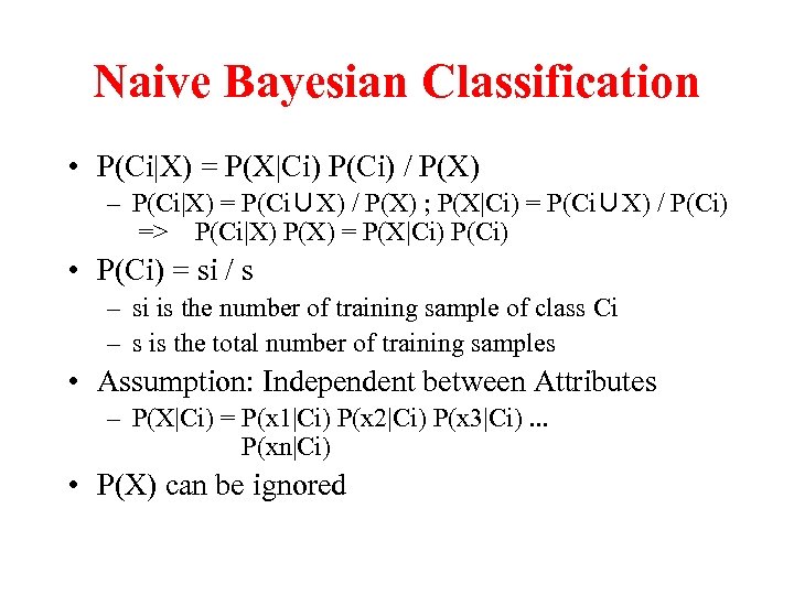Naive Bayesian Classification • P(Ci|X) = P(X|Ci) P(Ci) / P(X) – P(Ci|X) = P(Ci∪X) / P(X) ; P(X|Ci) = P(Ci∪X) / P(Ci) => P(Ci|X) P(X) = P(X|Ci) P(Ci) • P(Ci) = si / s – si is the number of training sample of class Ci – s is the total number of training samples • Assumption: Independent between Attributes – P(X|Ci) = P(x 1|Ci) P(x 2|Ci) P(x 3|Ci). . . P(xn|Ci) • P(X) can be ignored

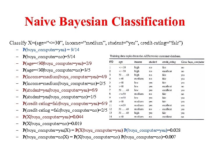Naive Bayesian Classification Classify X=(age=“<=30”, income=“medium”, student=“yes”, credit-rating=“fair”) – – – – P(buys_computer=yes) = 9/14 P(buys_computer=no)=5/14 P(age=<30|buys_computer=yes)=2/9 P(age=<30|buys_computer=no)=3/5 P(income=medium|buys_computer=yes)=4/9 P(income=medium|buys_computer=no)=2/5 P(student=yes|buys_computer=yes)=6/9 P(student=yes|buys_computer=no)=1/5 P(credit-rating=fair|buys_computer=yes)=6/9 P(credit-rating =fair|buys_computer=no)=2/5 P(X|buys_computer=yes)=0. 044 P(X|buys_computer=no)=0. 019 P(buys_computer=yes|X) = P(X|buys_computer=yes) P(buys_computer=yes)=0. 028 P(buys_computer=no|X) = P(X|buys_computer=no) P(buys_computer=no)=0. 007

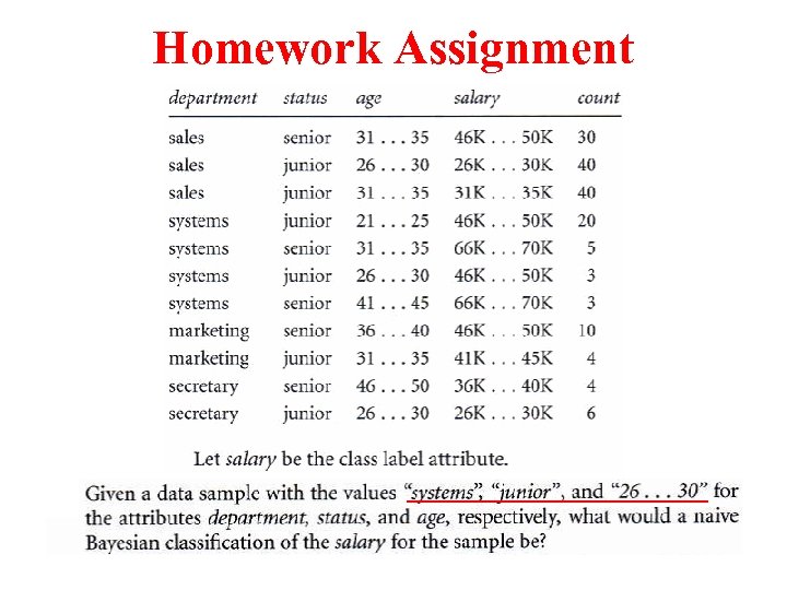Homework Assignment