Data Mining Lecture 12 Course Syllabus

Data Mining Lecture 12

Course Syllabus • Classification Techniques (Week 7 - Week 8 - Week 9) – – – Inductive Learning Decision Tree Learning Association Rules Neural Networks Regression Probabilistic Reasoning Bayesian Learning Lazy Learning Reinforcement Learning Genetic Algorithms Support Vector Machines Fuzzy Logic

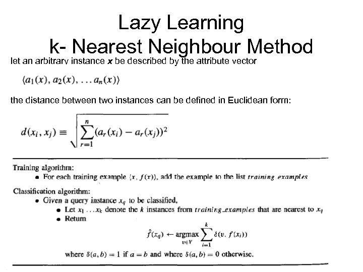
Lazy Learning k- Nearest Neighbour Method let an arbitrary instance x be described by the attribute vector the distance between two instances can be defined in Euclidean form:

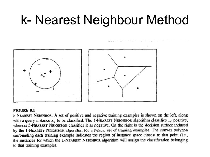
k- Nearest Neighbour Method

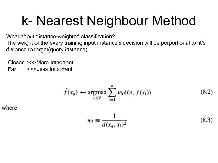
k- Nearest Neighbour Method What about distance-weighted classification? The weight of the every training input instance’s decision will be porportional to it’s distance to target(query instance) Closer >>>More Important Far >>>Less Important

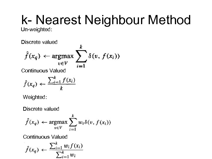
k- Nearest Neighbour Method Un-weighted: Discrete valued Continuous Valued Weighted: Discrete valued Continuous Valued

k- Nearest Neighbour Method – Curse of Dimensionality If the distance between neighbors will be dominated by the large number of irrelevant attributes then mis-calculation of distance occurs. This situation arises many irrelevant attributes are present, is sometimes referred to as the curse of dimensionality. Nearest-neighbor approaches are especially sensitive to this problem Solutions: Simply weigh attributes according to its importance Just ignore the irrelevant attributes

k- Nearest Neighbour Method – Lazy Learners Neighbouring Methods won’t learn till a classification problem arises. For every classification instance different decision making mechanism can be built. Thats why lazy learners can also be called as ”Local Learners” There is no training cost; but classification cost can be quite high Curse of dimensionality is another big problem

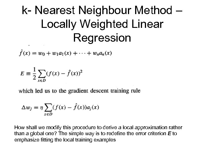
k- Nearest Neighbour Method – Locally Weighted Linear Regression How shall we modify this procedure to derive a local approximation rather than a global one? The simple way is to redefine the error criterion E to emphasize fitting the local training examples

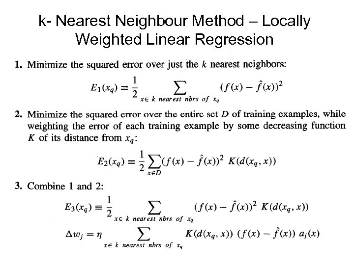
k- Nearest Neighbour Method – Locally Weighted Linear Regression

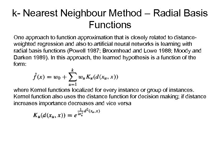
k- Nearest Neighbour Method – Radial Basis Functions One approach to function approximation that is closely related to distanceweighted regression and also to artificial neural networks is learning with radial basis functions (Powell 1987; Broomhead and Lowe 1988; Moody and Darken 1989). In this approach, the learned hypothesis is a function of the form: where Kernel functions localized for every instance or group of instances. Kernel function also uses the distance function for decision making; if distance increases importance decreases and vice versa

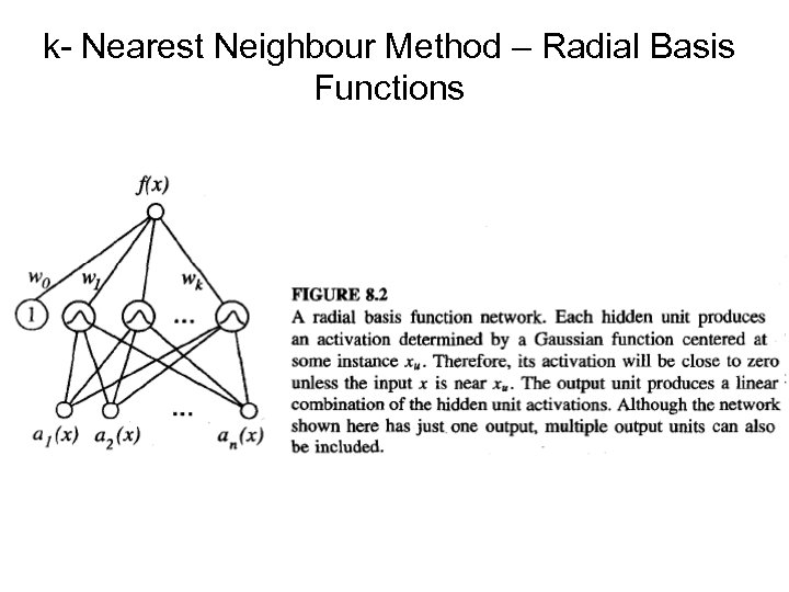
k- Nearest Neighbour Method – Radial Basis Functions

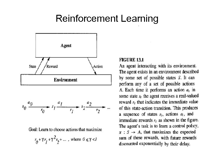
Reinforcement Learning

Reinforcement Learning • Reinforcement learning addresses the problem of learning control strategies for autonomous agents. It assumes that training information is available in the form of a real-valued reward signal given for each state-action transition. The goal of the agent is to learn an action policy that maximizes the total reward it will receive from any starting state • Markov decision processes, the outcome of applying any action to any state depends only on this action and state (and not on preceding actions: or states). Markov decision processes cover a wide range of problems including many robot control, factory automation, and scheduling problems.

Reinforcement Learning Reinforcement learning is closely related to dynamic programming approaches to Markov decision processes. The key difference is that historically these dynamic programming approaches have assumed that the agent possesses knowledge of the state transition function 6(s, a) and reward function r (s , a). In contrast, reinforcement learning algorithms such as Q learning typically assume the learner lacks such knowledge.

Genetic Algorithms - Models Of Evolution and Learning LAMARCKIAN EVOLUTION THEORY Lamarck was a scientist who, in the late nineteenth century, proposed that evolution over many generations was directly influenced by the experiences of individual organisms during their lifetime. In particular, he proposed that experiences of a single organism directly affected the genetic makeup of their offspring: If an individual learned during its lifetime to avoid some toxic food, it could pass this trait on genetically to its offspring, which therefore would not need to learn the trait

Genetic Algorithms - Models Of Evolution and Learning BALDWIN EFFECT If a species is evolving in a changing environment, there will be evolutionary pressure to favor individuals with the capability to learn during their lifetime. For example, if a new predator appears in the environment, then individuals capable of learning to avoid the predator will be more successful than individuals who cannot learn. In effect, the ability to learn allows an individual to perform a small local search during its lifetime to maximize its fitness. In contrast, nonlearning individuals whose fitness is fully determined by their genetic makeup will operate at a relative disadvantage. Those individuals who are able to learn many traits will rely less strongly on their genetic code to "hard-wire" traits. As a result, these individuals can support a more diverse gene pool, relying on individual learning to overcome the "missing" or "not quite optimized" traits in the genetic code. This more diverse gene pool can, in turn, support more rapid evolutionary adaptation. Thus, the ability of individuals to learn can have an indirect accelerating effect on the rate of evolutionary adaptation for the entire population.

Genetic Algorithms - Remarks Genetic algorithms (GAS) conduct controlled-randomized, parallel, hillclimbing search for hypotheses that optimize a predefined fitness function. GAS illustrate how learning can be viewed as a special case of optimization. In particular, the learning task is to find the optimal hypothesis, according to the predefined fitness function. This suggests that other optimization techniques such as simulated annealing can also be applied to machine learning problems. Genetic programming is a variant of genetic algorithms in which the hypotheses being manipulated are computer programs rather than bit strings. Operations such as crossover and mutation are generalized to apply to programs rather than bit strings. Genetic programming has been demonstrated to learn programs for tasks such as simulated robot control (Koza 1992) and recognizing objects in visual scenes (Teller and Veloso 1994).

Associations In data mining, association rule learning is a popular and well researched method for discovering interesting relations between variables in large databases. Piatetsky-Shapiro [1] describes analyzing and presenting strong rules discovered in databases using different measures of interestingness. Based on the concept of strong rules, Agrawal et al. [2] introduced association rules for discovering regularities between products in large scale transaction data recorded by point-of-sale (POS) systems in supermarkets. For example, the rule found in the sales data of a supermarket would indicate that if a customer buys onions and potatoes together, he or she is likely to also buy beef. Such information can be used as the basis for decisions about marketing activities such as, e. g. , promotional pricing or. In addition to the above example from market basket analysis association rules are employed today in many application areas including Web usage mining, intrusion detection and bioinformatics.

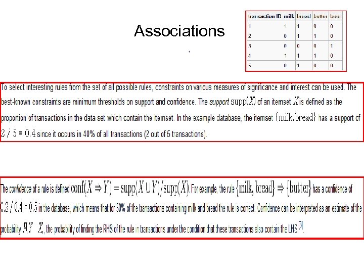
Associations

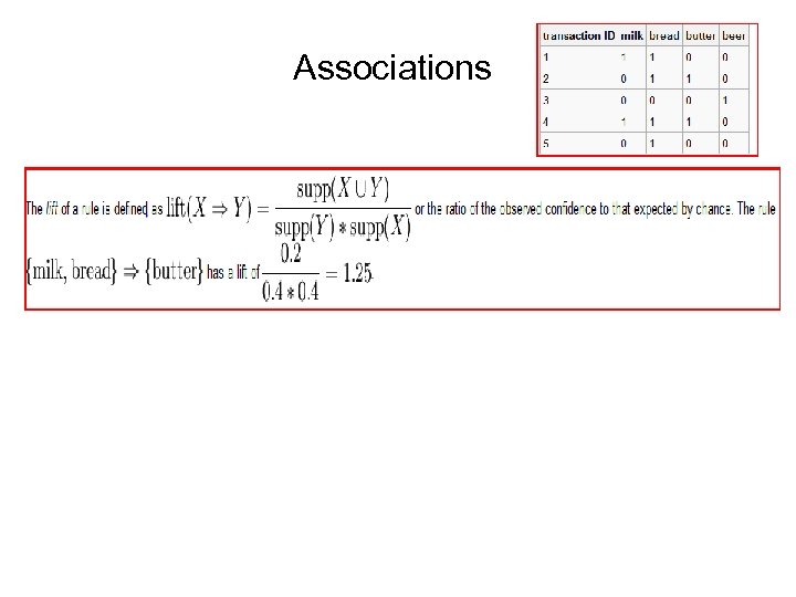
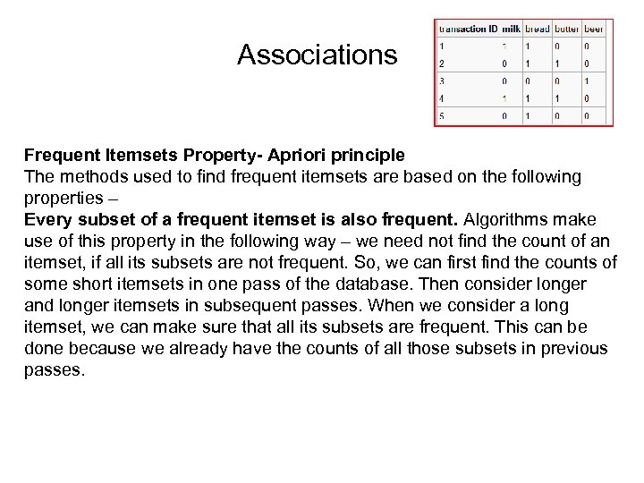
Associations Frequent Itemsets Property- Apriori principle The methods used to find frequent itemsets are based on the following properties – Every subset of a frequent itemset is also frequent. Algorithms make use of this property in the following way – we need not find the count of an itemset, if all its subsets are not frequent. So, we can first find the counts of some short itemsets in one pass of the database. Then consider longer and longer itemsets in subsequent passes. When we consider a long itemset, we can make sure that all its subsets are frequent. This can be done because we already have the counts of all those subsets in previous passes.

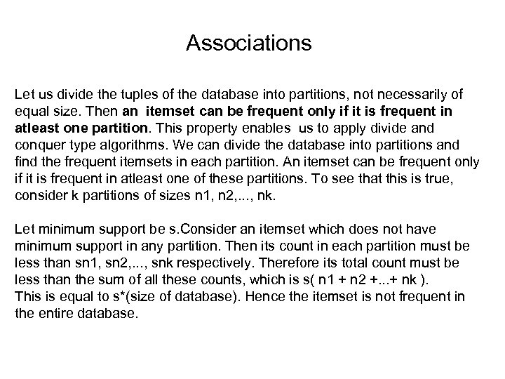
Associations Let us divide the tuples of the database into partitions, not necessarily of equal size. Then an itemset can be frequent only if it is frequent in atleast one partition. This property enables us to apply divide and conquer type algorithms. We can divide the database into partitions and find the frequent itemsets in each partition. An itemset can be frequent only if it is frequent in atleast one of these partitions. To see that this is true, consider k partitions of sizes n 1, n 2, . . . , nk. Let minimum support be s. Consider an itemset which does not have minimum support in any partition. Then its count in each partition must be less than sn 1, sn 2, . . . , snk respectively. Therefore its total count must be less than the sum of all these counts, which is s( n 1 + n 2 +. . . + nk ). This is equal to s*(size of database). Hence the itemset is not frequent in the entire database.

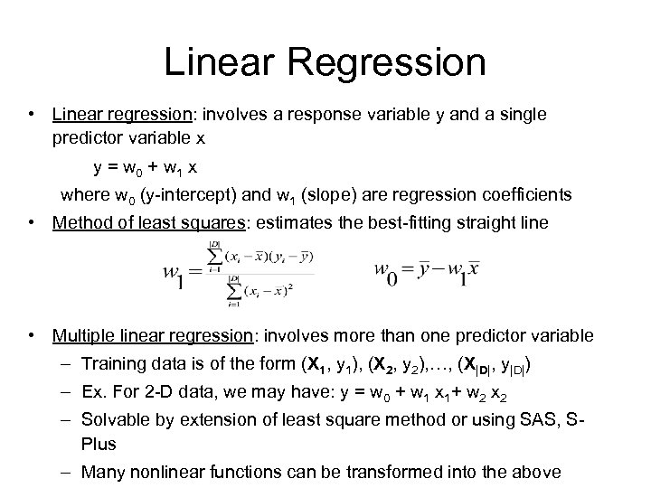
Linear Regression • Linear regression: involves a response variable y and a single predictor variable x y = w 0 + w 1 x where w 0 (y-intercept) and w 1 (slope) are regression coefficients • Method of least squares: estimates the best-fitting straight line • Multiple linear regression: involves more than one predictor variable – Training data is of the form (X 1, y 1), (X 2, y 2), …, (X|D|, y|D|) – Ex. For 2 -D data, we may have: y = w 0 + w 1 x 1+ w 2 x 2 – Solvable by extension of least square method or using SAS, SPlus – Many nonlinear functions can be transformed into the above

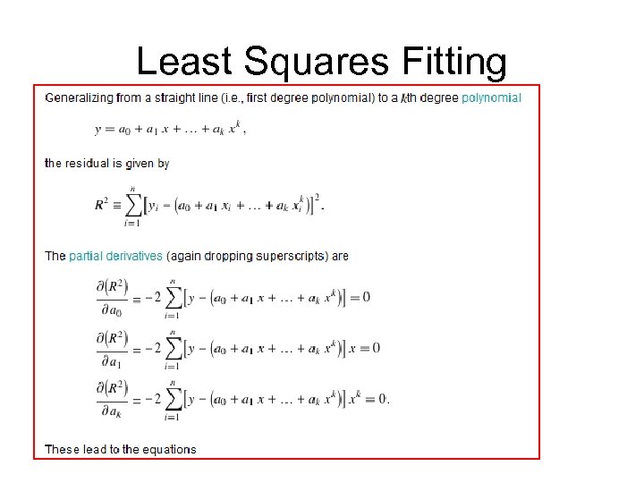
Least Squares Fitting

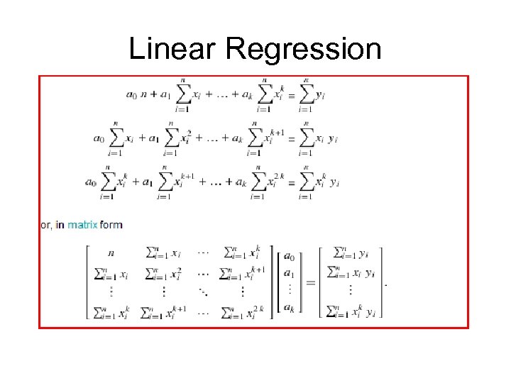
Linear Regression

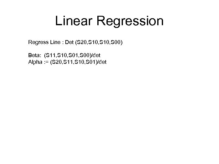
Linear Regression Regress Line : Det (S 20, S 10, S 00) Beta: (S 11, S 10, S 01, S 00)/det Alpha : = (S 20, S 11, S 10, S 01)/det

Nonlinear Regression • Some nonlinear models can be modeled by a polynomial function • A polynomial regression model can be transformed into linear regression model. For example, y = w 0 + w 1 x + w 2 x 2 + w 3 x 3 convertible to linear with new variables: x 2 = x 2, x 3= x 3 y = w 0 + w 1 x + w 2 x 2 + w 3 x 3 • Other functions, such as power function, can also be transformed to linear model • Some models are intractable nonlinear (e. g. , sum of exponential terms) – possible to obtain least square estimates through extensive calculation on more complex formulae

Other Regression-Based Models • Generalized linear model: – Foundation on which linear regression can be applied to modeling categorical response variables – Variance of y is a function of the mean value of y, not a constant – Logistic regression: models the prob. of some event occurring as a linear function of a set of predictor variables – Poisson regression: models the data that exhibit a Poisson distribution • Log-linear models: (for categorical data) – Approximate discrete multidimensional prob. distributions – Also useful for data compression and smoothing • Regression trees and model trees – Trees to predict continuous values rather than class labels

SVM—Support Vector Machines • A new classification method for both linear and nonlinear data • It uses a nonlinear mapping to transform the original training data into a higher dimension • With the new dimension, it searches for the linear optimal separating hyperplane (i. e. , “decision boundary”) • With an appropriate nonlinear mapping to a sufficiently high dimension, data from two classes can always be separated by a hyperplane • SVM finds this hyperplane using support vectors (“essential” training tuples) and margins (defined by the support vectors)

SVM—History and Applications • Vapnik and colleagues (1992)—groundwork from Vapnik & Chervonenkis’ statistical learning theory in 1960 s • Features: training can be slow but accuracy is high owing to their ability to model complex nonlinear decision boundaries (margin maximization) • Used both for classification and prediction • Applications: – handwritten digit recognition, object recognition, speaker identification, benchmarking time-series prediction tests

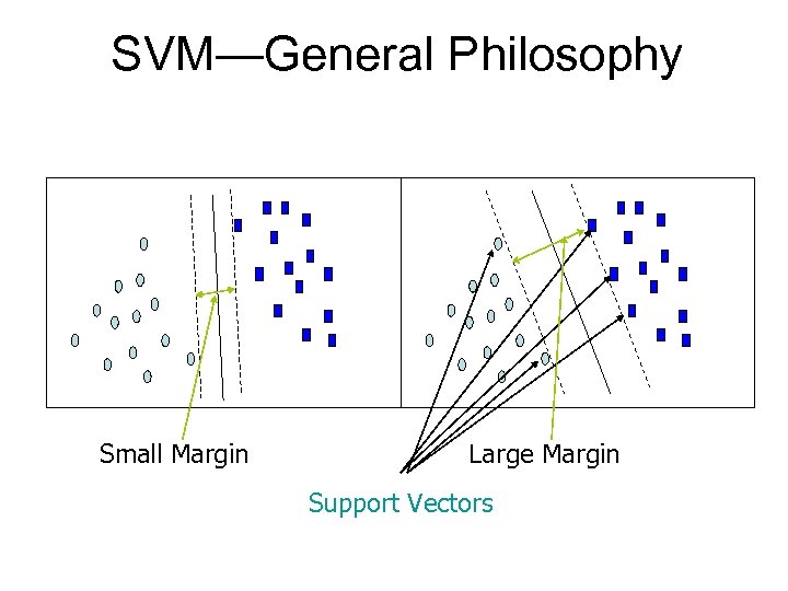
SVM—General Philosophy Small Margin Large Margin Support Vectors

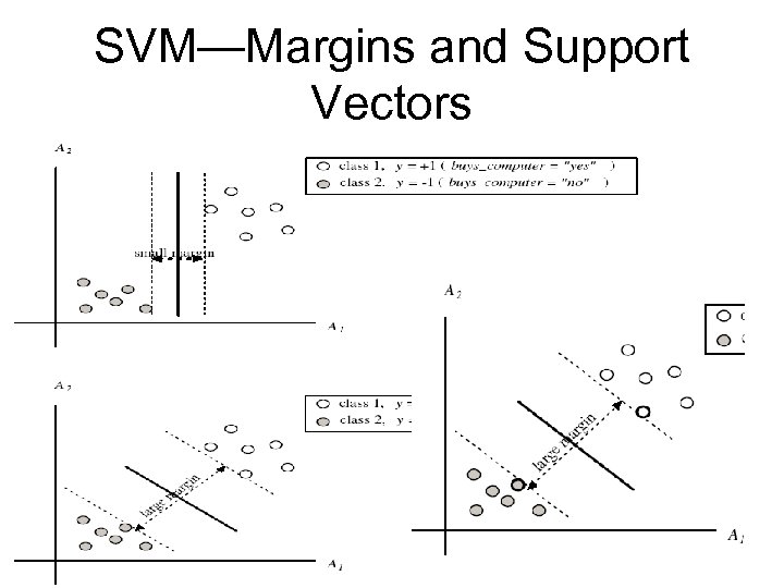
SVM—Margins and Support Vectors

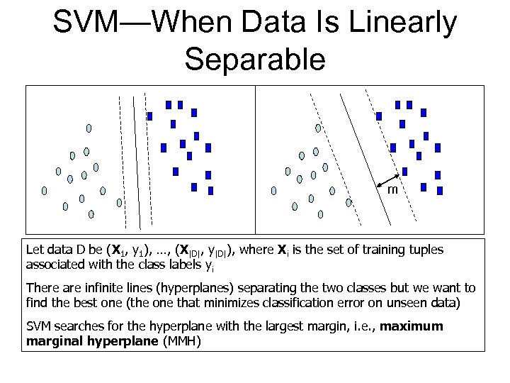
SVM—When Data Is Linearly Separable m Let data D be (X 1, y 1), …, (X|D|, y|D|), where Xi is the set of training tuples associated with the class labels yi There are infinite lines (hyperplanes) separating the two classes but we want to find the best one (the one that minimizes classification error on unseen data) SVM searches for the hyperplane with the largest margin, i. e. , maximum marginal hyperplane (MMH)

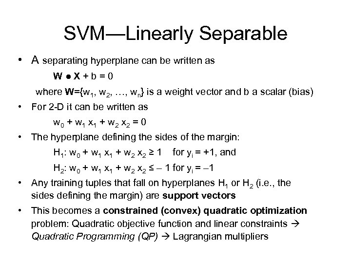
SVM—Linearly Separable • A separating hyperplane can be written as W●X+b=0 where W={w 1, w 2, …, wn} is a weight vector and b a scalar (bias) • For 2 -D it can be written as w 0 + w 1 x 1 + w 2 x 2 = 0 • The hyperplane defining the sides of the margin: H 1 : w 0 + w 1 x 1 + w 2 x 2 ≥ 1 for yi = +1, and H 2: w 0 + w 1 x 1 + w 2 x 2 ≤ – 1 for yi = – 1 • Any training tuples that fall on hyperplanes H 1 or H 2 (i. e. , the sides defining the margin) are support vectors • This becomes a constrained (convex) quadratic optimization problem: Quadratic objective function and linear constraints Quadratic Programming (QP) Lagrangian multipliers

Why Is SVM Effective on High Dimensional Data? • The complexity of trained classifier is characterized by the # of support vectors rather than the dimensionality of the data • The number of support vectors found can be used to compute an (upper) bound on the expected error rate of the SVM classifier, which is independent of the data dimensionality • Thus, an SVM with a small number of support vectors can have good generalization, even when the dimensionality of the data is high

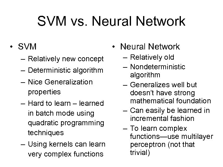
SVM vs. Neural Network • SVM – Relatively new concept – Deterministic algorithm – Nice Generalization properties – Hard to learn – learned in batch mode using quadratic programming techniques – Using kernels can learn very complex functions • Neural Network – Relatively old – Nondeterministic algorithm – Generalizes well but doesn’t have strong mathematical foundation – Can easily be learned in incremental fashion – To learn complex functions—use multilayer perceptron (not that trivial)

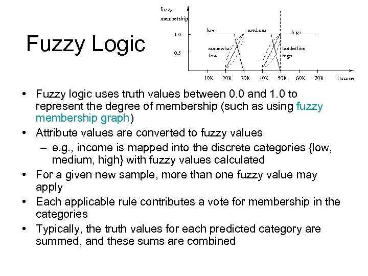
Fuzzy Logic • Fuzzy logic uses truth values between 0. 0 and 1. 0 to represent the degree of membership (such as using fuzzy membership graph) • Attribute values are converted to fuzzy values – e. g. , income is mapped into the discrete categories {low, medium, high} with fuzzy values calculated • For a given new sample, more than one fuzzy value may apply • Each applicable rule contributes a vote for membership in the categories • Typically, the truth values for each predicted category are summed, and these sums are combined

End of Lecture • read Chapter 6 of Course Text Book • read Chapter 6 – Supplemantary Text Book “Machine Learning” – Tom Mitchell