Data Mining Introduction Part of Lecture Notes for

Data Mining: Introduction Part of Lecture Notes for Introduction to Data Mining by Tan, Steinbach, Kumar © Tan, Steinbach, Kumar Introduction to Data Mining 4/18/2004 1

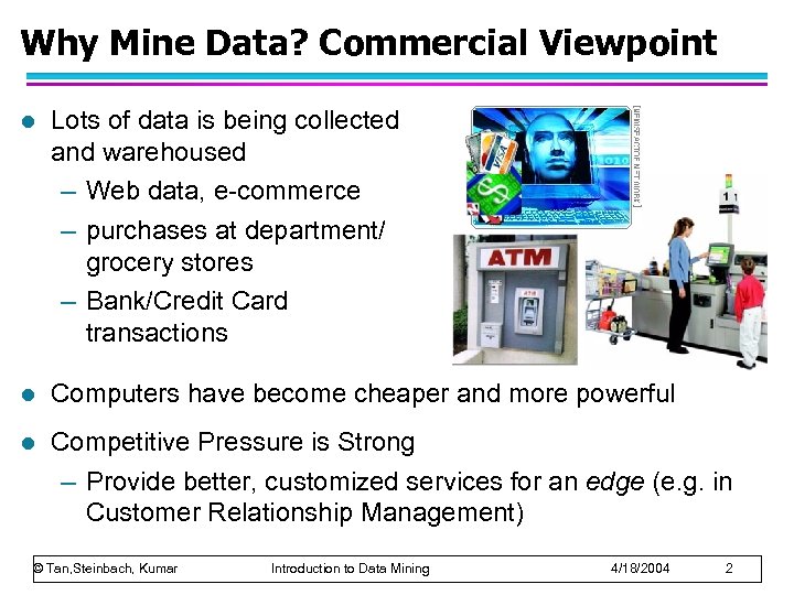Why Mine Data? Commercial Viewpoint l Lots of data is being collected and warehoused – Web data, e-commerce – purchases at department/ grocery stores – Bank/Credit Card transactions l Computers have become cheaper and more powerful l Competitive Pressure is Strong – Provide better, customized services for an edge (e. g. in Customer Relationship Management) © Tan, Steinbach, Kumar Introduction to Data Mining 4/18/2004 2

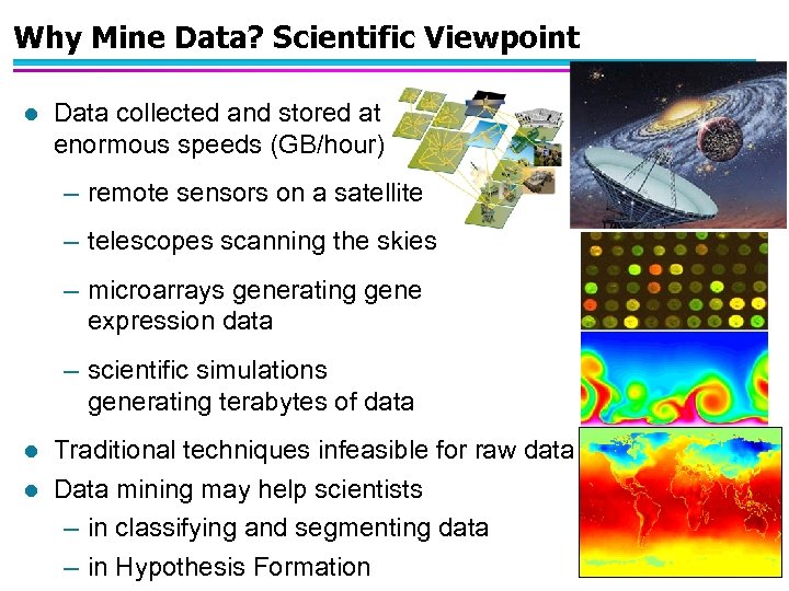Why Mine Data? Scientific Viewpoint l Data collected and stored at enormous speeds (GB/hour) – remote sensors on a satellite – telescopes scanning the skies – microarrays generating gene expression data – scientific simulations generating terabytes of data l l Traditional techniques infeasible for raw data Data mining may help scientists – in classifying and segmenting data – in Hypothesis Formation

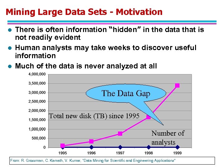Mining Large Data Sets - Motivation l l l There is often information “hidden” in the data that is not readily evident Human analysts may take weeks to discover useful information Much of the data is never analyzed at all The Data Gap Total new disk (TB) since 1995 Number of analysts © Tan, Steinbach, Kumar. Kamath, V. Kumar, “Data Mining for Scientific and Engineering Applications” From: R. Grossman, C. Introduction to Data Mining 4/18/2004 4

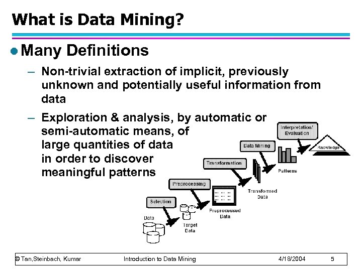What is Data Mining? l Many Definitions – Non-trivial extraction of implicit, previously unknown and potentially useful information from data – Exploration & analysis, by automatic or semi-automatic means, of large quantities of data in order to discover meaningful patterns © Tan, Steinbach, Kumar Introduction to Data Mining 4/18/2004 5

What is (not) Data Mining? What is not Data Mining? l – Look up phone number in phone directory – Query a Web search engine for information about “Amazon” © Tan, Steinbach, Kumar l What is Data Mining? – Certain names are more prevalent in certain US locations (O’Brien, O’Rurke, O’Reilly… in Boston area) – Group together similar documents returned by search engine according to their context (e. g. Amazon rainforest, Amazon. com, ) Introduction to Data Mining 4/18/2004 6

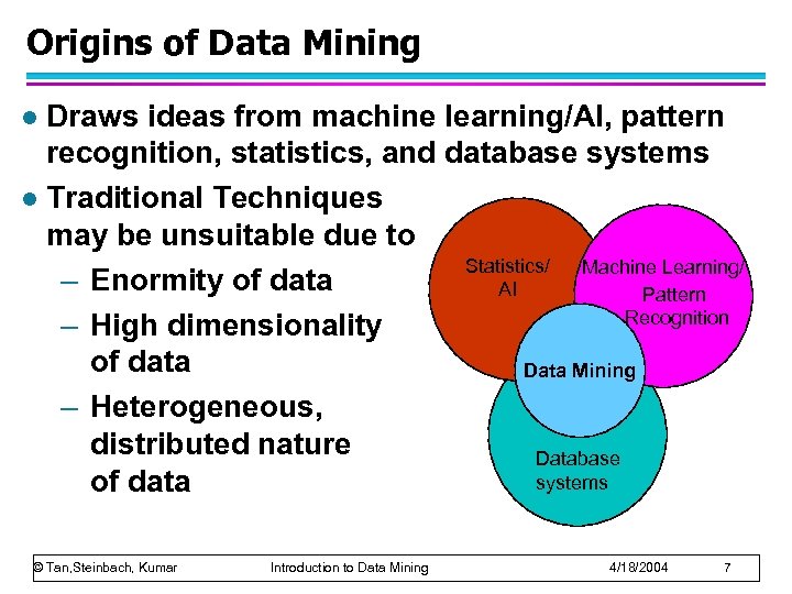Origins of Data Mining Draws ideas from machine learning/AI, pattern recognition, statistics, and database systems l Traditional Techniques may be unsuitable due to Statistics/ Machine Learning/ – Enormity of data AI Pattern Recognition – High dimensionality of data Data Mining – Heterogeneous, distributed nature Database systems of data l © Tan, Steinbach, Kumar Introduction to Data Mining 4/18/2004 7

Data Mining Tasks l Prediction Methods – Use some variables to predict unknown or future values of other variables. l Description Methods – Find human-interpretable patterns that describe the data. From [Fayyad, et. al. ] Advances in Knowledge Discovery and Data Mining, 1996 © Tan, Steinbach, Kumar Introduction to Data Mining 4/18/2004 8

Data Mining Tasks. . . Classification [Predictive] l Clustering [Descriptive] l Association Rule Discovery [Descriptive] l Sequential Pattern Discovery [Descriptive] l Regression [Predictive] l Deviation Detection [Predictive] l © Tan, Steinbach, Kumar Introduction to Data Mining 4/18/2004 9

Classification: Definition l Given a collection of records (training set ) – Each record contains a set of attributes, one of the attributes is the class. l l Find a model for class attribute as a function of the values of other attributes. Goal: previously unseen records should be assigned a class as accurately as possible. – A test set is used to determine the accuracy of the model. Usually, the given data set is divided into training and test sets, with training set used to build the model and test set used to validate it. © Tan, Steinbach, Kumar Introduction to Data Mining 4/18/2004 10

Classification Example l l a ic r o g te ca a ic r c in t on u uo s ss la c Test Set Training Set © Tan, Steinbach, Kumar Introduction to Data Mining Learn Classifier Model 4/18/2004 11

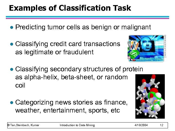Examples of Classification Task l Predicting tumor cells as benign or malignant l Classifying credit card transactions as legitimate or fraudulent l Classifying secondary structures of protein as alpha-helix, beta-sheet, or random coil l Categorizing news stories as finance, weather, entertainment, sports, etc © Tan, Steinbach, Kumar Introduction to Data Mining 4/18/2004 12

Classification: Application 1 l Direct Marketing – Goal: Reduce cost of mailing by targeting a set of consumers likely to buy a new cell-phone product. – Approach: u Use the data for a similar product introduced before. u We know which customers decided to buy and which decided otherwise. This {buy, don’t buy} decision forms the class attribute. u Collect various demographic, lifestyle, and companyinteraction related information about all such customers. – Type of business, where they stay, how much they earn, etc. u Use this information as input attributes to learn a classifier model. From [Berry & Linoff] Data Mining Techniques, 1997 © Tan, Steinbach, Kumar Introduction to Data Mining 4/18/2004 13

Classification: Application 2 l Fraud Detection – Goal: Predict fraudulent cases in credit card transactions. – Approach: u Use credit card transactions and the information on its account-holder as attributes. – When does a customer buy, what does he buy, how often he pays on time, etc u Label past transactions as fraud or fair transactions. This forms the class attribute. u Learn a model for the class of the transactions. u Use this model to detect fraud by observing credit card transactions on an account. © Tan, Steinbach, Kumar Introduction to Data Mining 4/18/2004 14

Classification: Application 3 l Customer Attrition/Churn: – Goal: To predict whether a customer is likely to be lost to a competitor. – Approach: u Use detailed record of transactions with each of the past and present customers, to find attributes. – How often the customer calls, where he calls, what time-of-the day he calls most, his financial status, marital status, etc. u Label the customers as loyal or disloyal. u Find a model for loyalty. From [Berry & Linoff] Data Mining Techniques, 1997 © Tan, Steinbach, Kumar Introduction to Data Mining 4/18/2004 15

Classification: Application 4 l Sky Survey Cataloging – Goal: To predict class (star or galaxy) of sky objects, especially visually faint ones, based on the telescopic survey images (from Palomar Observatory). – 3000 images with 23, 040 x 23, 040 pixels per image. – Approach: u Segment the image. u Measure image attributes (features) - 40 of them per object. u Model the class based on these features. u Success Story: Could find 16 new high red-shift quasars, some of the farthest objects that are difficult to find! From [Fayyad, et. al. ] Advances in Knowledge Discovery and Data Mining, 1996 © Tan, Steinbach, Kumar Introduction to Data Mining 4/18/2004 16

Classifying Galaxies Courtesy: http: //aps. umn. edu Early Class: • Stages of Formation Attributes: • Image features, • Characteristics of light waves received, etc. Intermediate Late Data Size: • 72 million stars, 20 million galaxies • Object Catalog: 9 GB • Image Database: 150 GB © Tan, Steinbach, Kumar Introduction to Data Mining 4/18/2004 17

Clustering Definition l l Given a set of data points, each having a set of attributes, and a similarity measure among them, find clusters such that – Data points in one cluster are more similar to one another. – Data points in separate clusters are less similar to one another. Similarity Measures: – Euclidean Distance if attributes are continuous. – Other Problem-specific Measures. © Tan, Steinbach, Kumar Introduction to Data Mining 4/18/2004 18

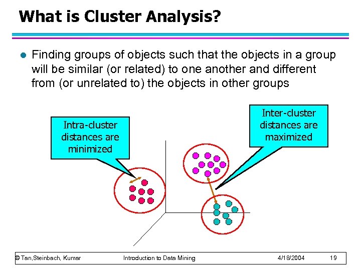What is Cluster Analysis? l Finding groups of objects such that the objects in a group will be similar (or related) to one another and different from (or unrelated to) the objects in other groups Inter-cluster distances are maximized Intra-cluster distances are minimized © Tan, Steinbach, Kumar Introduction to Data Mining 4/18/2004 19

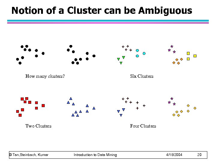Notion of a Cluster can be Ambiguous How many clusters? Six Clusters Two Clusters Four Clusters © Tan, Steinbach, Kumar Introduction to Data Mining 4/18/2004 20

Types of Clusterings l A clustering is a set of clusters l Important distinction between hierarchical and partitional sets of clusters l Partitional Clustering – A division data objects into non-overlapping subsets (clusters) such that each data object is in exactly one subset l Hierarchical clustering – A set of nested clusters organized as a hierarchical tree © Tan, Steinbach, Kumar Introduction to Data Mining 4/18/2004 21

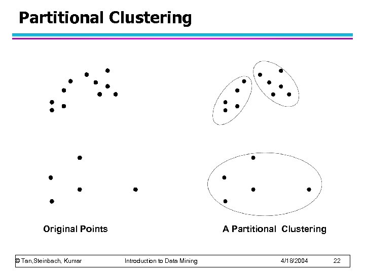Partitional Clustering Original Points © Tan, Steinbach, Kumar A Partitional Clustering Introduction to Data Mining 4/18/2004 22

Hierarchical Clustering Traditional Dendrogram Non-traditional Hierarchical Clustering Non-traditional Dendrogram © Tan, Steinbach, Kumar Introduction to Data Mining 4/18/2004 23

Types of Clusters l Well-separated clusters l Center-based clusters l Contiguous clusters l Density-based clusters l Property or Conceptual l Described by an Objective Function © Tan, Steinbach, Kumar Introduction to Data Mining 4/18/2004 24

Types of Clusters: Well-Separated l Well-Separated Clusters: – A cluster is a set of points such that any point in a cluster is closer (or more similar) to every other point in the cluster than to any point not in the cluster. 3 well-separated clusters © Tan, Steinbach, Kumar Introduction to Data Mining 4/18/2004 25

Types of Clusters: Center-Based l Center-based – A cluster is a set of objects such that an object in a cluster is closer (more similar) to the “center” of a cluster, than to the center of any other cluster – The center of a cluster is often a centroid, the average of all the points in the cluster, or a medoid, the most “representative” point of a cluster 4 center-based clusters © Tan, Steinbach, Kumar Introduction to Data Mining 4/18/2004 26

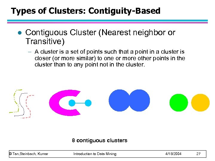Types of Clusters: Contiguity-Based l Contiguous Cluster (Nearest neighbor or Transitive) – A cluster is a set of points such that a point in a cluster is closer (or more similar) to one or more other points in the cluster than to any point not in the cluster. 8 contiguous clusters © Tan, Steinbach, Kumar Introduction to Data Mining 4/18/2004 27

Types of Clusters: Density-Based l Density-based – A cluster is a dense region of points, which is separated by low -density regions, from other regions of high density. – Used when the clusters are irregular or intertwined, and when noise and outliers are present. 6 density-based clusters © Tan, Steinbach, Kumar Introduction to Data Mining 4/18/2004 28

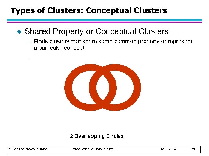Types of Clusters: Conceptual Clusters l Shared Property or Conceptual Clusters – Finds clusters that share some common property or represent a particular concept. . 2 Overlapping Circles © Tan, Steinbach, Kumar Introduction to Data Mining 4/18/2004 29

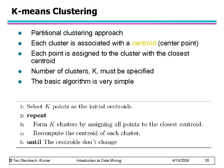K-means Clustering l Partitional clustering approach l Each cluster is associated with a centroid (center point) l Each point is assigned to the cluster with the closest centroid l Number of clusters, K, must be specified l The basic algorithm is very simple © Tan, Steinbach, Kumar Introduction to Data Mining 4/18/2004 30

K-means Clustering – Details l Initial centroids are often chosen randomly. – Clusters produced vary from one run to another. l The centroid is (typically) the mean of the points in the cluster. l ‘Closeness’ is measured by Euclidean distance, cosine similarity, correlation, etc. l K-means will converge for common similarity measures mentioned above. l Most of the convergence happens in the first few iterations. – l Often the stopping condition is changed to ‘Until relatively few points change clusters’ Complexity is O( n * K * I * d ) – n = number of points, K = number of clusters, I = number of iterations, d = number of attributes © Tan, Steinbach, Kumar Introduction to Data Mining 4/18/2004 31

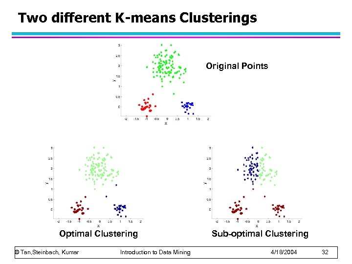Two different K-means Clusterings Original Points Optimal Clustering © Tan, Steinbach, Kumar Introduction to Data Mining Sub-optimal Clustering 4/18/2004 32

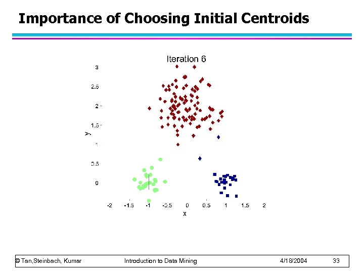Importance of Choosing Initial Centroids © Tan, Steinbach, Kumar Introduction to Data Mining 4/18/2004 33

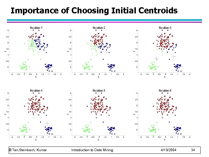Importance of Choosing Initial Centroids © Tan, Steinbach, Kumar Introduction to Data Mining 4/18/2004 34

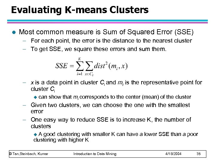Evaluating K-means Clusters l Most common measure is Sum of Squared Error (SSE) – For each point, the error is the distance to the nearest cluster – To get SSE, we square these errors and sum them. – x is a data point in cluster Ci and mi is the representative point for cluster Ci u can show that mi corresponds to the center (mean) of the cluster – Given two clusters, we can choose the one with the smallest error – One easy way to reduce SSE is to increase K, the number of clusters A good clustering with smaller K can have a lower SSE than a poor clustering with higher K u © Tan, Steinbach, Kumar Introduction to Data Mining 4/18/2004 35

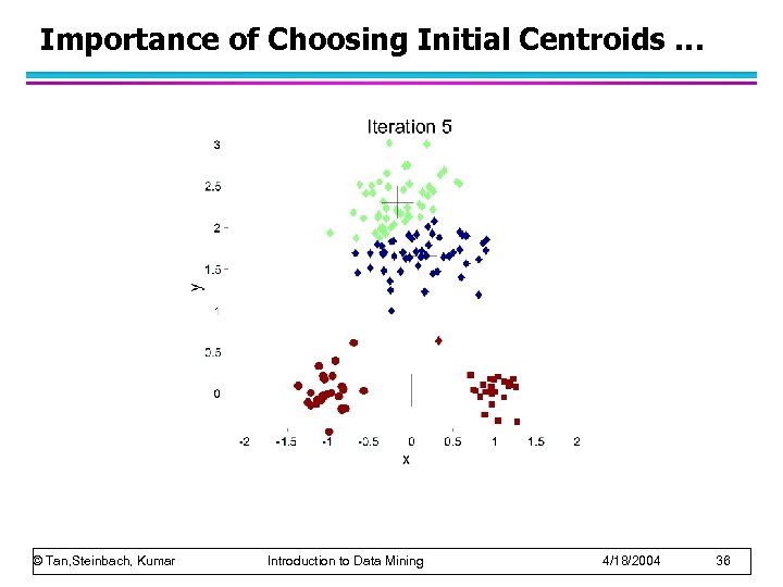Importance of Choosing Initial Centroids … © Tan, Steinbach, Kumar Introduction to Data Mining 4/18/2004 36

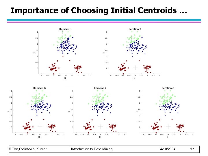Importance of Choosing Initial Centroids … © Tan, Steinbach, Kumar Introduction to Data Mining 4/18/2004 37

Problems with Selecting Initial Points l If there are K ‘real’ clusters then the chance of selecting one centroid from each cluster is small. – – Chance is relatively small when K is large – – For example, if K = 10, then probability = 10!/1010 = 0. 00036 – Consider an example of five pairs of clusters If clusters are the same size, n, then Sometimes the initial centroids will readjust themselves in ‘right’ way, and sometimes they don’t © Tan, Steinbach, Kumar Introduction to Data Mining 4/18/2004 38

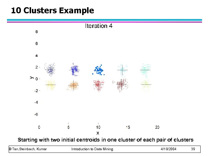10 Clusters Example Starting with two initial centroids in one cluster of each pair of clusters © Tan, Steinbach, Kumar Introduction to Data Mining 4/18/2004 39

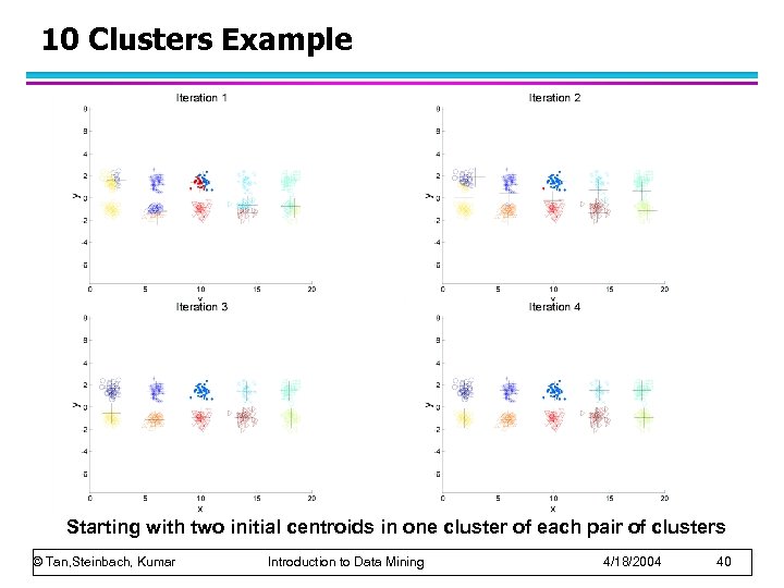10 Clusters Example Starting with two initial centroids in one cluster of each pair of clusters © Tan, Steinbach, Kumar Introduction to Data Mining 4/18/2004 40

10 Clusters Example Starting with some pairs of clusters having three initial centroids, while other have only one. © Tan, Steinbach, Kumar Introduction to Data Mining 4/18/2004 41

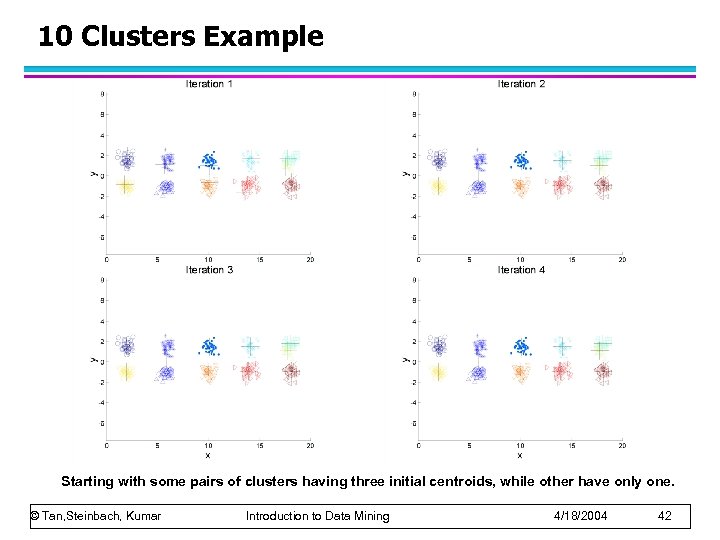10 Clusters Example Starting with some pairs of clusters having three initial centroids, while other have only one. © Tan, Steinbach, Kumar Introduction to Data Mining 4/18/2004 42

Solutions to Initial Centroids Problem Multiple runs – Helps, but probability is not on your side l Sample and use hierarchical clustering to determine initial centroids l Select more than k initial centroids and then select among these initial centroids – Select most widely separated l Postprocessing l Bisecting K-means – Not as susceptible to initialization issues l © Tan, Steinbach, Kumar Introduction to Data Mining 4/18/2004 43

Hierarchical Clustering Produces a set of nested clusters organized as a hierarchical tree l Can be visualized as a dendrogram – A tree like diagram that records the sequences of merges or splits l © Tan, Steinbach, Kumar Introduction to Data Mining 4/18/2004 44

Strengths of Hierarchical Clustering l Do not have to assume any particular number of clusters – Any desired number of clusters can be obtained by ‘cutting’ the dendogram at the proper level l They may correspond to meaningful taxonomies – Example in biological sciences (e. g. , animal kingdom, phylogeny reconstruction, …) © Tan, Steinbach, Kumar Introduction to Data Mining 4/18/2004 45

Hierarchical Clustering l Two main types of hierarchical clustering – Agglomerative: u Start with the points as individual clusters At each step, merge the closest pair of clusters until only one cluster (or k clusters) left u – Divisive: u Start with one, all-inclusive cluster At each step, split a cluster until each cluster contains a point (or there are k clusters) u l Traditional hierarchical algorithms use a similarity or distance matrix – Merge or split one cluster at a time © Tan, Steinbach, Kumar Introduction to Data Mining 4/18/2004 46

Agglomerative Clustering Algorithm l More popular hierarchical clustering technique l Basic algorithm is straightforward 1. 2. 3. 4. 5. 6. l Compute the proximity matrix Let each data point be a cluster Repeat Merge the two closest clusters Update the proximity matrix Until only a single cluster remains Key operation is the computation of the proximity of two clusters – Different approaches to defining the distance between clusters distinguish the different algorithms © Tan, Steinbach, Kumar Introduction to Data Mining 4/18/2004 47

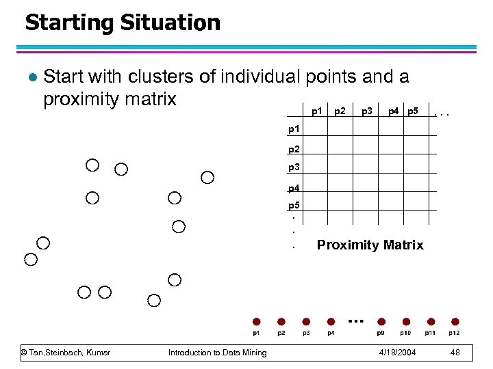Starting Situation l Start with clusters of individual points and a proximity matrix p 1 p 2 p 3 p 4 p 5 . . . p 1 p 2 p 3 p 4 p 5. . . © Tan, Steinbach, Kumar Introduction to Data Mining Proximity Matrix 4/18/2004 48

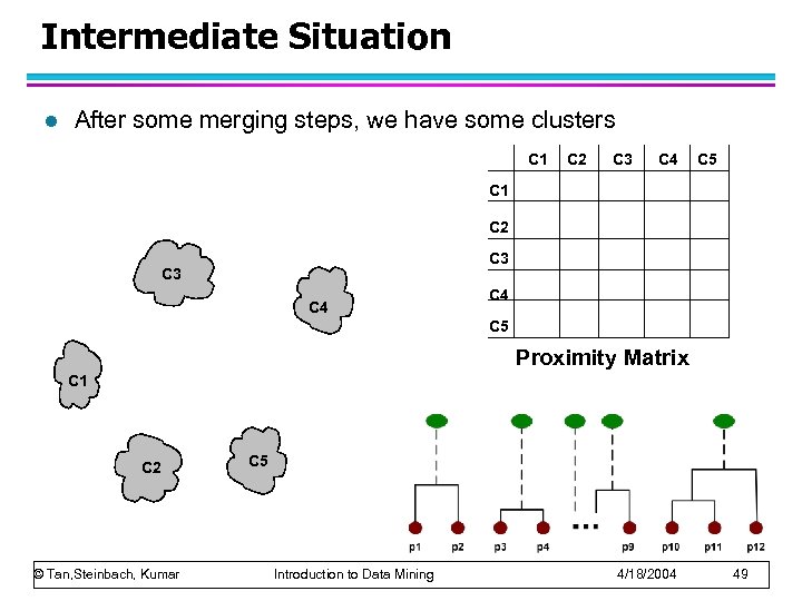Intermediate Situation l After some merging steps, we have some clusters C 1 C 2 C 3 C 4 C 5 Proximity Matrix C 1 C 2 © Tan, Steinbach, Kumar C 5 Introduction to Data Mining 4/18/2004 49

Intermediate Situation l We want to merge the two closest clusters (C 2 and C 5) and update the proximity matrix. C 1 C 2 C 3 C 4 C 5 Proximity Matrix C 1 C 2 © Tan, Steinbach, Kumar C 5 Introduction to Data Mining 4/18/2004 50

After Merging l The question is “How do we update the proximity matrix? ” C 1 C 2 U C 5 C 3 C 2 U C 5 C 4 ? ? ? C 3 ? C 4 C 3 ? Proximity Matrix C 1 C 2 U C 5 © Tan, Steinbach, Kumar Introduction to Data Mining 4/18/2004 51

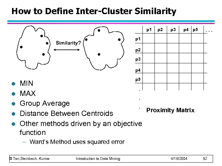How to Define Inter-Cluster Similarity p 1 Similarity? p 2 p 3 p 4 p 5 . . . p 1 p 2 p 3 p 4 l l l p 5 MIN. MAX. Group Average. Proximity Matrix Distance Between Centroids Other methods driven by an objective function – Ward’s Method uses squared error © Tan, Steinbach, Kumar Introduction to Data Mining 4/18/2004 52

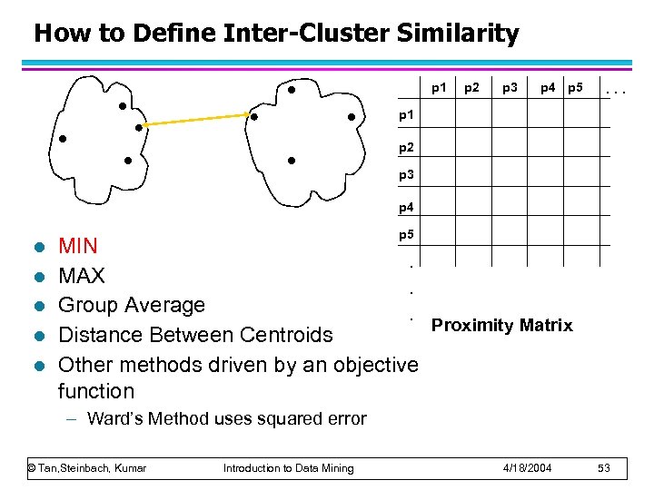How to Define Inter-Cluster Similarity p 1 p 2 p 3 p 4 p 5 . . . p 1 p 2 p 3 p 4 l l l p 5 MIN. MAX. Group Average. Proximity Matrix Distance Between Centroids Other methods driven by an objective function – Ward’s Method uses squared error © Tan, Steinbach, Kumar Introduction to Data Mining 4/18/2004 53

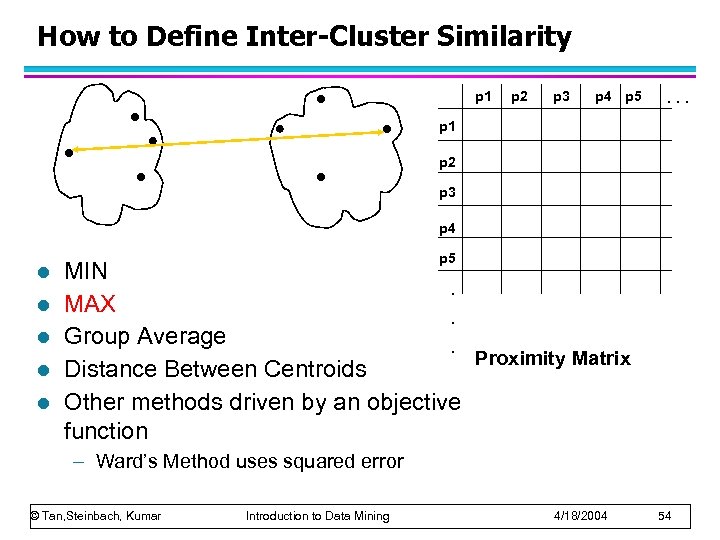How to Define Inter-Cluster Similarity p 1 p 2 p 3 p 4 p 5 . . . p 1 p 2 p 3 p 4 l l l p 5 MIN. MAX. Group Average. Proximity Matrix Distance Between Centroids Other methods driven by an objective function – Ward’s Method uses squared error © Tan, Steinbach, Kumar Introduction to Data Mining 4/18/2004 54

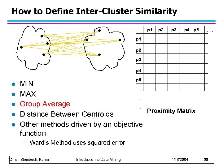How to Define Inter-Cluster Similarity p 1 p 2 p 3 p 4 p 5 . . . p 1 p 2 p 3 p 4 l l l p 5 MIN. MAX. Group Average. Proximity Matrix Distance Between Centroids Other methods driven by an objective function – Ward’s Method uses squared error © Tan, Steinbach, Kumar Introduction to Data Mining 4/18/2004 55

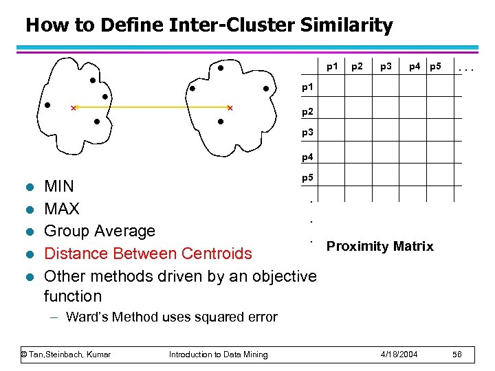How to Define Inter-Cluster Similarity p 1 p 2 p 3 p 4 p 5 . . . p 1 p 2 p 3 p 4 l l l p 5 MIN. MAX. Group Average. Proximity Matrix Distance Between Centroids Other methods driven by an objective function – Ward’s Method uses squared error © Tan, Steinbach, Kumar Introduction to Data Mining 4/18/2004 56

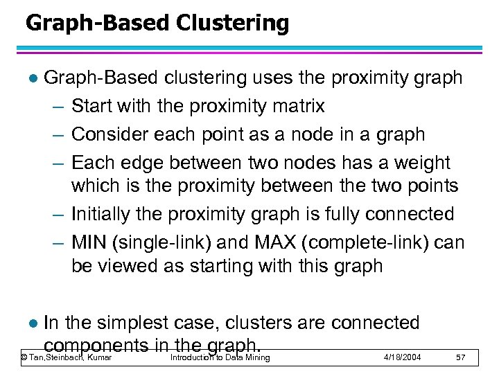Graph-Based Clustering l Graph-Based clustering uses the proximity graph – Start with the proximity matrix – Consider each point as a node in a graph – Each edge between two nodes has a weight which is the proximity between the two points – Initially the proximity graph is fully connected – MIN (single-link) and MAX (complete-link) can be viewed as starting with this graph In the simplest case, clusters are connected components in Introduction to Data Mining the graph. © Tan, Steinbach, Kumar 4/18/2004 l 57

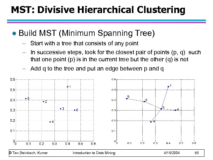MST: Divisive Hierarchical Clustering l Build MST (Minimum Spanning Tree) – Start with a tree that consists of any point – In successive steps, look for the closest pair of points (p, q) such that one point (p) is in the current tree but the other (q) is not – Add q to the tree and put an edge between p and q © Tan, Steinbach, Kumar Introduction to Data Mining 4/18/2004 58

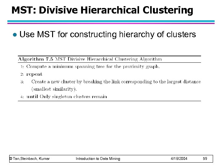MST: Divisive Hierarchical Clustering l Use MST for constructing hierarchy of clusters © Tan, Steinbach, Kumar Introduction to Data Mining 4/18/2004 59

Clustering: Application 1 l Market Segmentation: – Goal: subdivide a market into distinct subsets of customers where any subset may conceivably be selected as a market target to be reached with a distinct marketing mix. – Approach: u Collect different attributes of customers based on their geographical and lifestyle related information. u Find clusters of similar customers. u Measure the clustering quality by observing buying patterns of customers in same cluster vs. those from different clusters. © Tan, Steinbach, Kumar Introduction to Data Mining 4/18/2004 60

Clustering: Application 2 l Document Clustering: – Goal: To find groups of documents that are similar to each other based on the important terms appearing in them. – Approach: To identify frequently occurring terms in each document. Form a similarity measure based on the frequencies of different terms. Use it to cluster. – Gain: Information Retrieval can utilize the clusters to relate a new document or search term to clustered documents. © Tan, Steinbach, Kumar Introduction to Data Mining 4/18/2004 61

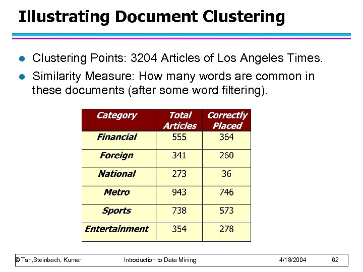Illustrating Document Clustering l l Clustering Points: 3204 Articles of Los Angeles Times. Similarity Measure: How many words are common in these documents (after some word filtering). © Tan, Steinbach, Kumar Introduction to Data Mining 4/18/2004 62

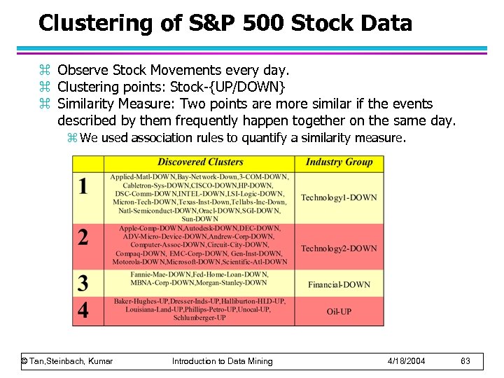Clustering of S&P 500 Stock Data z Observe Stock Movements every day. z Clustering points: Stock-{UP/DOWN} z Similarity Measure: Two points are more similar if the events described by them frequently happen together on the same day. z We used association rules to quantify a similarity measure. © Tan, Steinbach, Kumar Introduction to Data Mining 4/18/2004 63

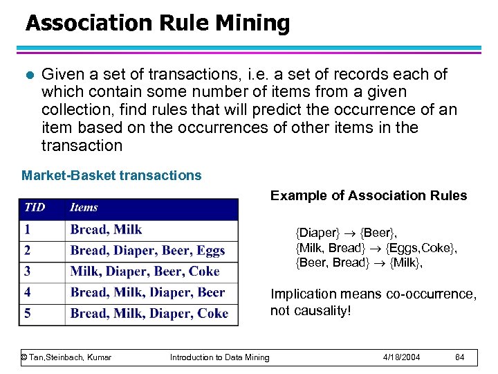Association Rule Mining l Given a set of transactions, i. e. a set of records each of which contain some number of items from a given collection, find rules that will predict the occurrence of an item based on the occurrences of other items in the transaction Market-Basket transactions Example of Association Rules {Diaper} {Beer}, {Milk, Bread} {Eggs, Coke}, {Beer, Bread} {Milk}, Implication means co-occurrence, not causality! © Tan, Steinbach, Kumar Introduction to Data Mining 4/18/2004 64

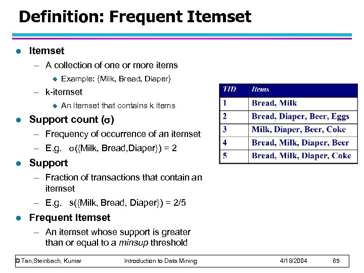Definition: Frequent Itemset l Itemset – A collection of one or more items u Example: {Milk, Bread, Diaper} – k-itemset u l An itemset that contains k items Support count ( ) – Frequency of occurrence of an itemset – E. g. ({Milk, Bread, Diaper}) = 2 l Support – Fraction of transactions that contain an itemset – E. g. s({Milk, Bread, Diaper}) = 2/5 l Frequent Itemset – An itemset whose support is greater than or equal to a minsup threshold © Tan, Steinbach, Kumar Introduction to Data Mining 4/18/2004 65

Definition: Association Rule l Association Rule – An implication expression of the form X Y, where X and Y are itemsets – Example: {Milk, Diaper} {Beer} l Rule Evaluation Metrics – Support (s) u Fraction of transactions that contain both X and Y Example: – Confidence (c) u Measures how often items in Y appear in transactions that contain X © Tan, Steinbach, Kumar Introduction to Data Mining 4/18/2004 66

Association Rule Mining Task l Given a set of transactions T, the goal of association rule mining is to find all rules having – support ≥ minsup threshold – confidence ≥ minconf threshold l Brute-force approach: – List all possible association rules – Compute support and confidence for each rule – Prune rules that fail the minsup and minconf thresholds Computationally prohibitive! © Tan, Steinbach, Kumar Introduction to Data Mining 4/18/2004 67

Mining Association Rules Example of Rules: {Milk, Diaper} {Beer} (s=0. 4, c=0. 67) {Milk, Beer} {Diaper} (s=0. 4, c=1. 0) {Diaper, Beer} {Milk} (s=0. 4, c=0. 67) {Beer} {Milk, Diaper} (s=0. 4, c=0. 67) {Diaper} {Milk, Beer} (s=0. 4, c=0. 5) {Milk} {Diaper, Beer} (s=0. 4, c=0. 5) Observations: • All the above rules are binary partitions of the same itemset: {Milk, Diaper, Beer} • Rules originating from the same itemset have identical support but can have different confidence • Thus, we may decouple the support and confidence requirements © Tan, Steinbach, Kumar Introduction to Data Mining 4/18/2004 68

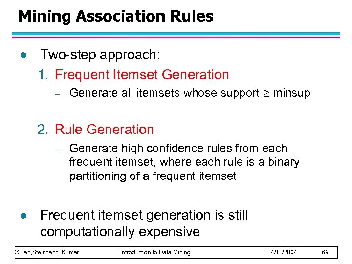Mining Association Rules l Two-step approach: 1. Frequent Itemset Generation – Generate all itemsets whose support minsup 2. Rule Generation – l Generate high confidence rules from each frequent itemset, where each rule is a binary partitioning of a frequent itemset Frequent itemset generation is still computationally expensive © Tan, Steinbach, Kumar Introduction to Data Mining 4/18/2004 69

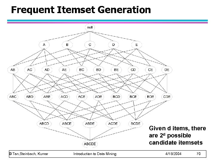Frequent Itemset Generation Given d items, there are 2 d possible candidate itemsets © Tan, Steinbach, Kumar Introduction to Data Mining 4/18/2004 70

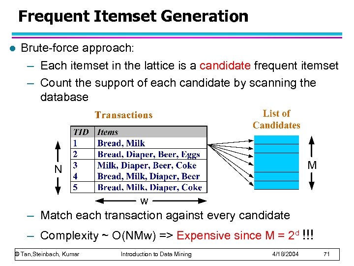Frequent Itemset Generation l Brute-force approach: – Each itemset in the lattice is a candidate frequent itemset – Count the support of each candidate by scanning the database – Match each transaction against every candidate – Complexity ~ O(NMw) => Expensive since M = 2 d !!! © Tan, Steinbach, Kumar Introduction to Data Mining 4/18/2004 71

Computational Complexity l Given d unique items: – Total number of itemsets = 2 d – Total number of possible association rules: If d=6, R = 602 rules © Tan, Steinbach, Kumar Introduction to Data Mining 4/18/2004 72

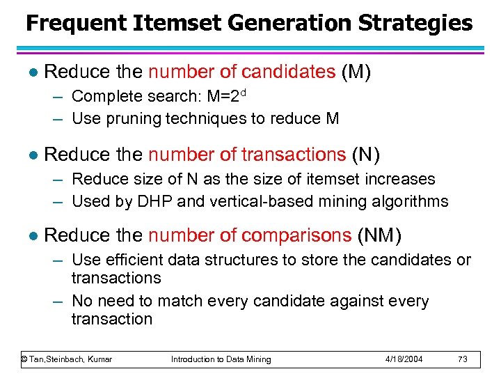Frequent Itemset Generation Strategies l Reduce the number of candidates (M) – Complete search: M=2 d – Use pruning techniques to reduce M l Reduce the number of transactions (N) – Reduce size of N as the size of itemset increases – Used by DHP and vertical-based mining algorithms l Reduce the number of comparisons (NM) – Use efficient data structures to store the candidates or transactions – No need to match every candidate against every transaction © Tan, Steinbach, Kumar Introduction to Data Mining 4/18/2004 73

Reducing Number of Candidates l Apriori principle: – If an itemset is frequent, then all of its subsets must also be frequent l Apriori principle holds due to the following property of the support measure: – Support of an itemset never exceeds the support of its subsets – This is known as the anti-monotone property of support © Tan, Steinbach, Kumar Introduction to Data Mining 4/18/2004 74

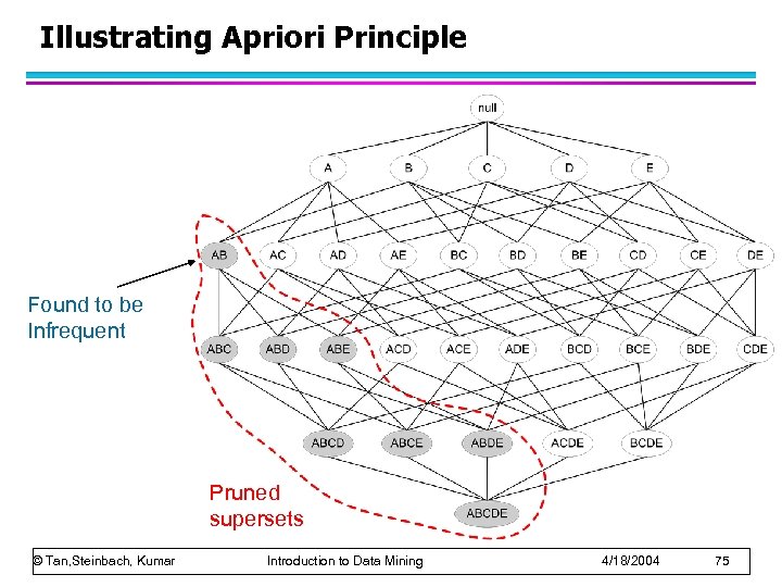Illustrating Apriori Principle Found to be Infrequent Pruned supersets © Tan, Steinbach, Kumar Introduction to Data Mining 4/18/2004 75

Illustrating Apriori Principle Items (1 -itemsets) Pairs (2 -itemsets) (No need to generate candidates involving Coke or Eggs) Minimum Support = 3 Triplets (3 -itemsets) If every subset is considered, 6 C + 6 C = 41 1 2 3 With support-based pruning, 6 + 1 = 13 © Tan, Steinbach, Kumar Introduction to Data Mining 4/18/2004 76

Apriori Algorithm l Method: – Let k=1 – Generate frequent itemsets of length 1 – Repeat until no new frequent itemsets are identified u Generate length (k+1) candidate itemsets from length k frequent itemsets u Prune candidate itemsets containing subsets of length k that are infrequent u Count the support of each candidate by scanning the DB u Eliminate candidates that are infrequent, leaving only those that are frequent © Tan, Steinbach, Kumar Introduction to Data Mining 4/18/2004 77

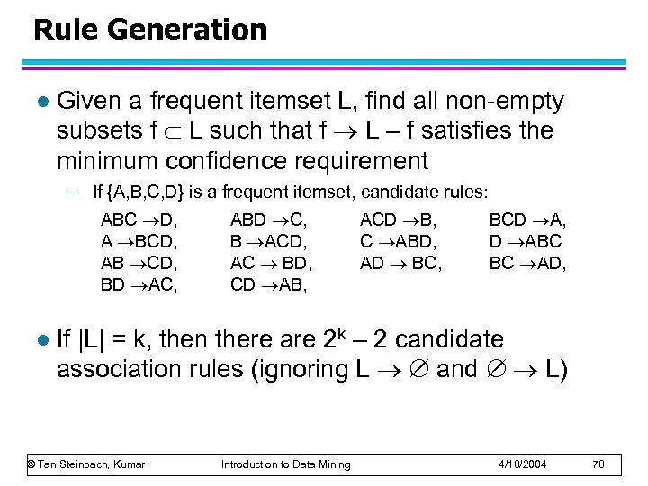Rule Generation l Given a frequent itemset L, find all non-empty subsets f L such that f L – f satisfies the minimum confidence requirement – If {A, B, C, D} is a frequent itemset, candidate rules: ABC D, ABD C, ACD B, BCD A, A BCD, B ACD, C ABD, D ABC AB CD, AC BD, AD BC, BC AD, BD AC, CD AB, l If |L| = k, then there are 2 k – 2 candidate association rules (ignoring L and L) © Tan, Steinbach, Kumar Introduction to Data Mining 4/18/2004 78

Rule Generation l How to efficiently generate rules from frequent itemsets? – In general, confidence does not have an antimonotone property c(ABC D) can be larger or smaller than c(AB D) – But confidence of rules generated from the same itemset has an anti-monotone property – e. g. , L = {A, B, C, D}: c(ABC D) c(AB CD) c(A BCD) u Confidence is anti-monotone w. r. t. number of items on the RHS of the rule © Tan, Steinbach, Kumar Introduction to Data Mining 4/18/2004 79

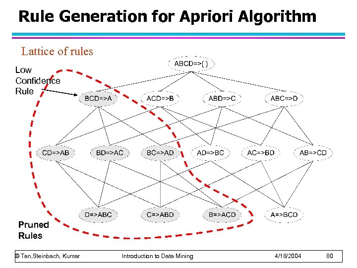Rule Generation for Apriori Algorithm Lattice of rules Low Confidence Rule Pruned Rules © Tan, Steinbach, Kumar Introduction to Data Mining 4/18/2004 80

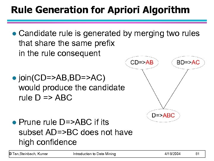Rule Generation for Apriori Algorithm l Candidate rule is generated by merging two rules that share the same prefix in the rule consequent l join(CD=>AB, BD=>AC) would produce the candidate rule D => ABC l Prune rule D=>ABC if its subset AD=>BC does not have high confidence © Tan, Steinbach, Kumar Introduction to Data Mining 4/18/2004 81

Association Rule Discovery: Application 1 l Marketing and Sales Promotion: – Let the rule discovered be {Bagels, … } --> {Potato Chips} – Potato Chips as consequent => Can be used to determine what should be done to boost its sales. – Bagels in the antecedent => Can be used to see which products would be affected if the store discontinues selling bagels. – Bagels in antecedent and Potato chips in consequent => Can be used to see what products should be sold with Bagels to promote sale of Potato chips! © Tan, Steinbach, Kumar Introduction to Data Mining 4/18/2004 82

Association Rule Discovery: Application 2 l Supermarket shelf management. – Goal: To identify items that are bought together by sufficiently many customers. – Approach: Process the point-of-sale data collected with barcode scanners to find dependencies among items. – A classic rule -u If a customer buys diaper and milk, then he is very likely to buy beer. u So, don’t be surprised if you find six-packs stacked next to diapers! © Tan, Steinbach, Kumar Introduction to Data Mining 4/18/2004 83

Association Rule Discovery: Application 3 l Inventory Management: – Goal: A consumer appliance repair company wants to anticipate the nature of repairs on its consumer products and keep the service vehicles equipped with right parts to reduce on number of visits to consumer households. – Approach: Process the data on tools and parts required in previous repairs at different consumer locations and discover the co-occurrence patterns. © Tan, Steinbach, Kumar Introduction to Data Mining 4/18/2004 84

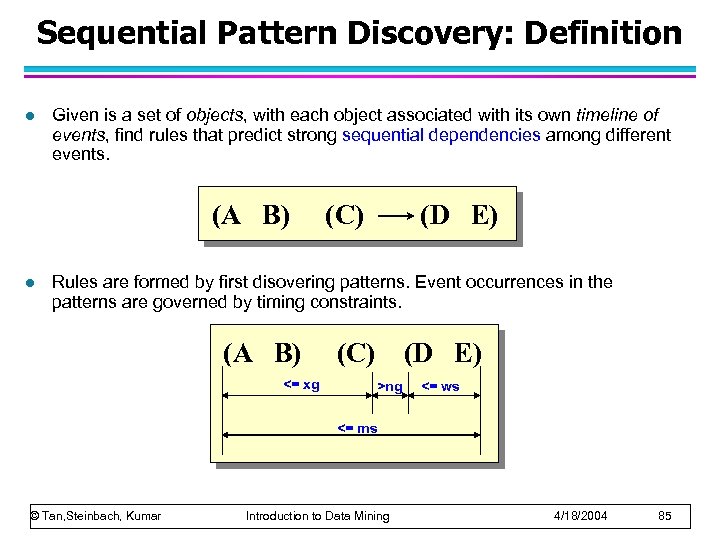Sequential Pattern Discovery: Definition l Given is a set of objects, with each object associated with its own timeline of events, find rules that predict strong sequential dependencies among different events. (A B) l (C) (D E) Rules are formed by first disovering patterns. Event occurrences in the patterns are governed by timing constraints. (A B) <= xg (C) (D E) >ng <= ws <= ms © Tan, Steinbach, Kumar Introduction to Data Mining 4/18/2004 85

Sequential Pattern Discovery: Examples l l In telecommunications alarm logs, – (Inverter_Problem Excessive_Line_Current) (Rectifier_Alarm) --> (Fire_Alarm) In point-of-sale transaction sequences, – Computer Bookstore: (Intro_To_Visual_C) (C++_Primer) --> (Perl_for_dummies, Tcl_Tk) – Athletic Apparel Store: (Shoes) (Racket, Racketball) --> (Sports_Jacket) © Tan, Steinbach, Kumar Introduction to Data Mining 4/18/2004 86

Regression l l l Predict a value of a given continuous valued variable based on the values of other variables, assuming a linear or nonlinear model of dependency. Greatly studied in statistics, neural network fields. Examples: – Predicting sales amounts of new product based on advetising expenditure. – Predicting wind velocities as a function of temperature, humidity, air pressure, etc. – Time series prediction of stock market indices. © Tan, Steinbach, Kumar Introduction to Data Mining 4/18/2004 87

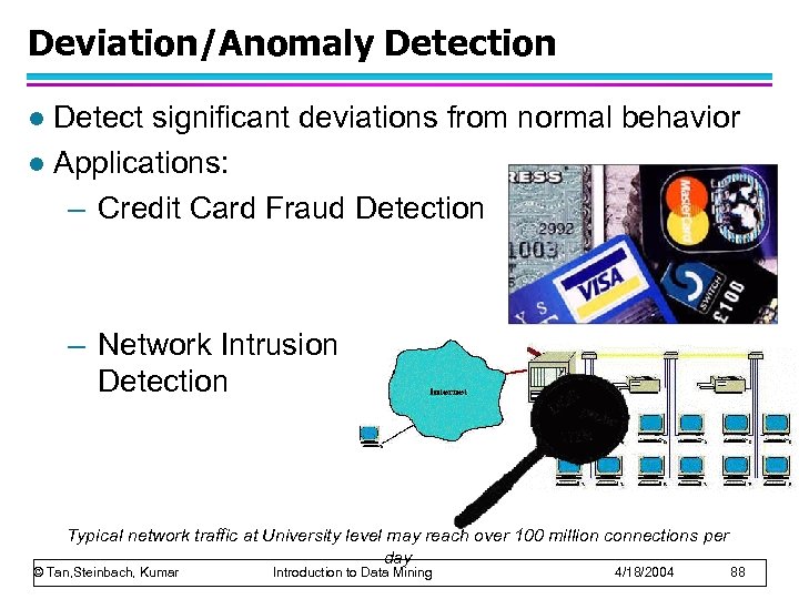Deviation/Anomaly Detection Detect significant deviations from normal behavior l Applications: – Credit Card Fraud Detection l – Network Intrusion Detection Typical network traffic at University level may reach over 100 million connections per day © Tan, Steinbach, Kumar Introduction to Data Mining 4/18/2004 88

Challenges of Data Mining l l l l Scalability Dimensionality Complex and Heterogeneous Data Quality Data Ownership and Distribution Privacy Preservation Streaming Data © Tan, Steinbach, Kumar Introduction to Data Mining 4/18/2004 89