Data Mining in Market Research What is

Data Mining in Market Research • What is data mining? – Methods for finding interesting structure in large databases • E. g. patterns, prediction rules, unusual cases – Focus on efficient, scalable algorithms • Contrasts with emphasis on correct inference in statistics – Related to data warehousing, machine learning • Why is data mining important? – Well marketed; now a large industry; pays well – Handles large databases directly – Can make data analysis more accessible to end users • Semi-automation of analysis • Results can be easier to interpret than e. g. regression models • Strong focus on decisions and their implementation

Data Mining Software • Many providers of data mining software – SAS Enterprise Miner, SPSS Clementine, Statistica Data Miner, MS SQL Server, Polyanalyst, Knowledge. STUDIO, … – See http: //www. kdnuggets. com/software/suites. html for a list – Good algorithms important, but also need good facilities for handling data and meta-data • Recommend: – WEKA (Waikato Environment for Knowledge Analysis) • Free (GPLed) Java package with GUI • Online at www. cs. waikato. ac. nz/ml/weka • Witten and Frank, 2000. Data Mining: Practical Machine Learning Tools and Techniques with Java Implementations. – R packages • E. g. rpart, class, tree, nnet, cclust, deal, Gene. SOM, knn. Tree, mlbench, random. Forest, subselect

Data Mining Terms • Different names for familiar statistical concepts, from database and AI communities – Observation = case, record, instance – Variable = field, attribute – Analysis of dependence vs interdependence = Supervised vs unsupervised learning – Relationship = association, concept – Dependent variable = response, output – Independent variable = predictor, input

Common Data Mining Techniques • Predictive modeling – Classification • Derive classification rules • Decision trees – Numeric prediction • Regression trees, model trees • Association rules • Meta-learning methods – Cross-validation, bagging, boosting • Other data mining methods include: – artificial neural networks, genetic algorithms, density estimation, clustering, abstraction, discretisation, visualisation, detecting changes in data or models

Classification • Methods for predicting a discrete response – One kind of supervised learning – Note: in biological and other sciences, classification has long had a different meaning, referring to cluster analysis • Applications include: – Identifying good prospects for specific marketing or sales efforts • Cross-selling, up-selling – when to offer products • Customers likely to be especially profitable • Customers likely to defect – Identifying poor credit risks – Diagnosing customer problems

Weather/Game-Playing Data • Small dataset – 14 instances – 5 attributes • • • Outlook - nominal Temperature - numeric Humidity - numeric Wind - nominal Play – Whether or not a certain game would be played – This is what we want to understand predict

ARFF file for the weather data.

German Credit Risk Dataset • 1000 instances (people), 21 attributes – “class” attribute describes people as good or bad credit risks – Other attributes include financial information and demographics • E. g. checking_status, duration, credit_history, purpose, credit_amount, savings_status, employment, Age, housing, job, num_dependents, own_telephone, foreign_worker • Want to predict credit risk • Data available at UCI machine learning data repository • http: //www. ics. uci. edu/~mlearn/MLRepository. html

Classification Algorithms • Many methods available in WEKA – 0 R, 1 R, Naive. Bayes, Decision. Table, ID 3, PRISM, Instance-based learner (IB 1, IBk), C 4. 5 (J 48), PART, Support vector machine (SMO) • Usually train on part of the data, test on the rest • Simple method – Zero-rule, or 0 R – Predict the most common category • Class Zero. R in WEKA – Too simple for practical use, but a useful baseline for evaluating performance of more complex methods

1 -Rule (1 R) Algorithm • Based on single predictor – Predict mode within each value of that predictor • Look at error rate for each predictor on training dataset, and choose best predictor • Called One. R in WEKA • Must group numerical predictor values for this method – Common method is to split at each change in the response – Collapse buckets until each contains at least 6 instances

1 R Algorithm (continued) • Biased towards predictors with more categories – These can result in over-fitting to the training data • But found to perform surprisingly well – Study on 16 widely used datasets • Holte (1993), Machine Learning 11, 63 -91 – Often error rate only a few percentages points higher than more sophisticated methods (e. g. decision trees) – Produced rules that were much simpler and more easily understood

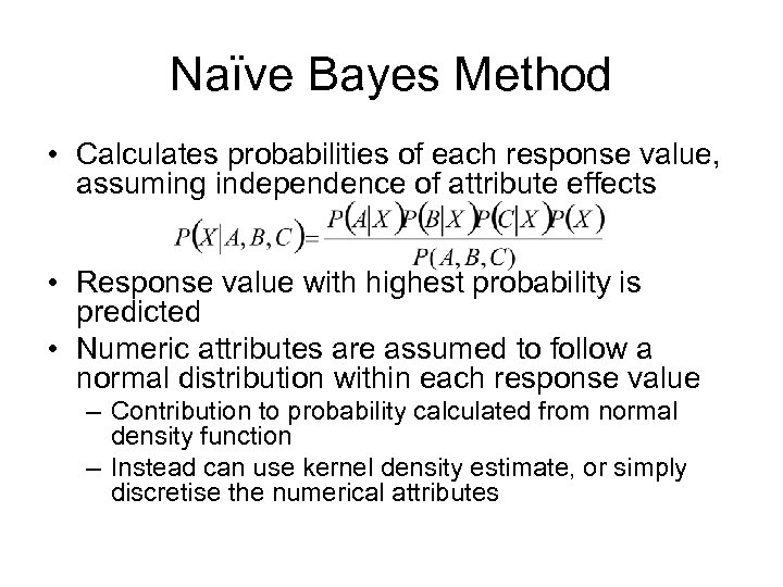Naïve Bayes Method • Calculates probabilities of each response value, assuming independence of attribute effects • Response value with highest probability is predicted • Numeric attributes are assumed to follow a normal distribution within each response value – Contribution to probability calculated from normal density function – Instead can use kernel density estimate, or simply discretise the numerical attributes

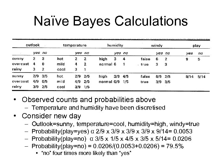Naïve Bayes Calculations • Observed counts and probabilities above – Temperature and humidity have been discretised • Consider new day – – Outlook=sunny, temperature=cool, humidity=high, windy=true Probability(play=yes) α 2/9 x 3/9 x 9/14= 0. 0053 Probability(play=no) α 3/5 x 1/5 x 4/5 x 3/5 x 5/14= 0. 0206 Probability(play=no) = 0. 0206/(0. 0053+0. 0206) = 79. 5% • “no” four times more likely than “yes”

Naïve Bayes Method • If any of the component probabilities are zero, the whole probability is zero – Effectively a veto on that response value – Add one to each cell’s count to get around this problem • Corresponds to weak positive prior information • Naïve Bayes effectively assumes that attributes are equally important – Several highly correlated attributes could drown out an important variable that would add new information • However this method often works well in practice

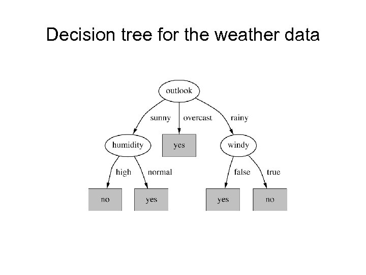
Decision Trees • Classification rules can be expressed in a tree structure – Move from the top of the tree, down through various nodes, to the leaves – At each node, a decision is made using a simple test based on attribute values – The leaf you reach holds the appropriate predicted value • Decision trees are appealing and easily used – However they can be verbose – Depending on the tests being used, they may obscure rather than reveal the true pattern • More info online at http: //recursive-partitioning. com/

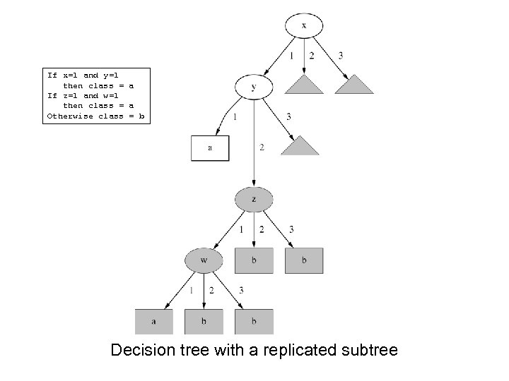If x=1 and y=1 then class = a If z=1 and w=1 then class = a Otherwise class = b Decision tree with a replicated subtree

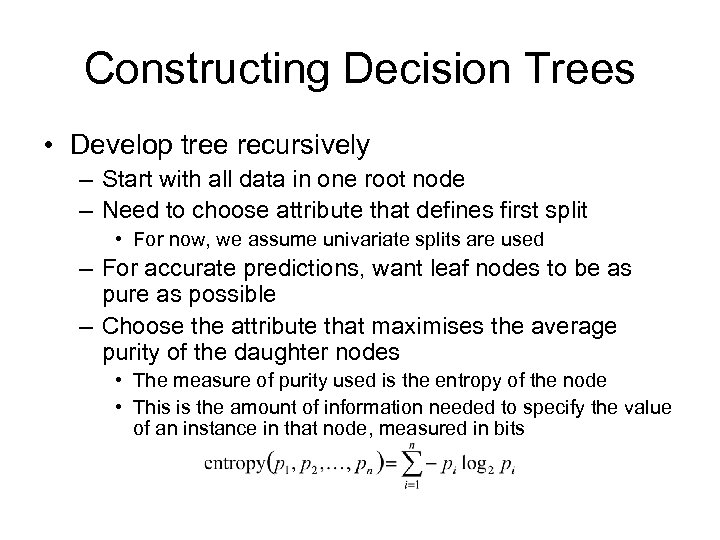Constructing Decision Trees • Develop tree recursively – Start with all data in one root node – Need to choose attribute that defines first split • For now, we assume univariate splits are used – For accurate predictions, want leaf nodes to be as pure as possible – Choose the attribute that maximises the average purity of the daughter nodes • The measure of purity used is the entropy of the node • This is the amount of information needed to specify the value of an instance in that node, measured in bits

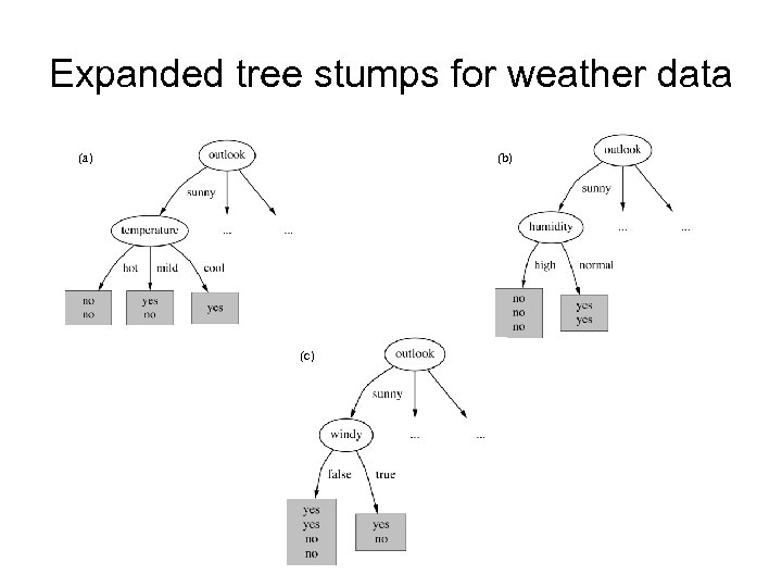
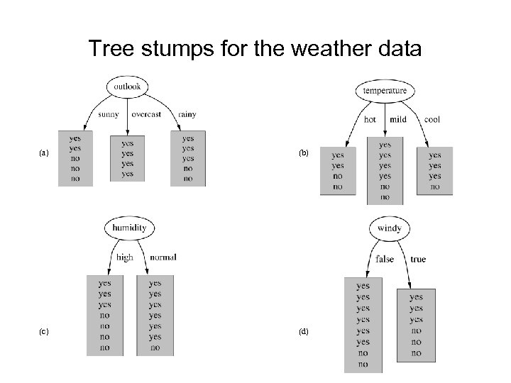Tree stumps for the weather data (a) (b) (c) (d)

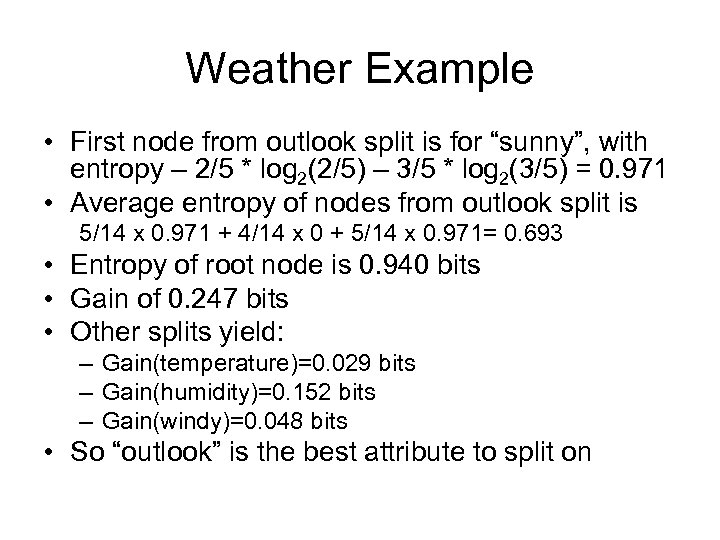Weather Example • First node from outlook split is for “sunny”, with entropy – 2/5 * log 2(2/5) – 3/5 * log 2(3/5) = 0. 971 • Average entropy of nodes from outlook split is 5/14 x 0. 971 + 4/14 x 0 + 5/14 x 0. 971= 0. 693 • Entropy of root node is 0. 940 bits • Gain of 0. 247 bits • Other splits yield: – Gain(temperature)=0. 029 bits – Gain(humidity)=0. 152 bits – Gain(windy)=0. 048 bits • So “outlook” is the best attribute to split on

Expanded tree stumps for weather data (a) (b) (c)

Decision tree for the weather data

Decision Tree Algorithms • The algorithm described in the preceding slides is known as ID 3 – Due to Quinlan (1986) • Tends to choose attributes with many values – Using information gain ratio helps solve this problem • Several more improvements have been made to handle numeric attributes (via univariate splits), missing values and noisy data (via pruning) – Resulting algorithm known as C 4. 5 • Described by Quinlan (1993) – Widely used (as is the commercial version C 5. 0) – WEKA has a version called J 4. 8

Classification Trees • Described (along with regression trees) in: – L. Breiman, J. H. Friedman, R. A. Olshen, and C. J. Stone, 1984. Classification and Regression Trees. • More sophisticated method than ID 3 – However Quinlan’s (1993) C 4. 5 method caught up with CART in most areas • CART also incorporates methods for pruning, missing values and numeric attributes – Multivariate splits are possible, as well as univariate • Split on linear combination Σcjxj > d – CART typically uses Gini measure of node purity to determine best splits • This is of the form Σp(1 -p) – But information/entropy measure also available

Regression Trees • Trees can also be used to predict numeric attributes – Predict using average value of the response in the appropriate node • Implemented in CART and C 4. 5 frameworks – Can use a model at each node instead • Implemented in Weka’s M 5’ algorithm • Harder to interpret than regression trees • Classification and regression trees are implemented in R’s rpart package – See Ch 10 in Venables and Ripley, MASS 3 rd Ed.

Problems with Trees • Can be unnecessarily verbose • Structure often unstable – “Greedy” hierarchical algorithm • Small variations can change chosen splits at high level nodes, which then changes subtree below • Conclusions about attribute importance can be unreliable • Direct methods tend to over fit training dataset – This problem can be reduced by pruning the tree • Another approach that often works well is to fit the tree, remove all training cases that are not correctly predicted, and refit the tree on the reduced dataset – Typically gives a smaller tree – This usually works almost as well on the training data – But generalises better, e. g. works better on test data • Bagging the tree algorithm also gives more stable results – Will discuss bagging later

Classification Tree Example • Example Weka’s J 4. 8 algorithm on German credit data (with default options) – 1000 instances, 21 attributes • Produces a pruned tree with 140 nodes, 103 leaves

• === Run information === • • Scheme: weka. classifiers. j 48. J 48 -C 0. 25 -M 2 Relation: german_credit Instances: 1000 Attributes: 21 • Number of Leaves : 103 • Size of the tree : 140 • • === Stratified cross-validation === Summary === • • Correctly Classified Instances 739 73. 9 % Incorrectly Classified Instances 261 26. 1 % Kappa statistic 0. 3153 Mean absolute error 0. 3241 Root mean squared error 0. 4604 Relative absolute error 77. 134 % Root relative squared error 100. 4589 % Total Number of Instances 1000 • === Detailed Accuracy By Class === • • • TP Rate FP Rate Precision Recall F-Measure Class 0. 883 0. 597 0. 775 0. 883 0. 826 good 0. 403 0. 117 0. 596 0. 403 0. 481 bad • === Confusion Matrix === • • • a b <-- classified as 618 82 | a = good 179 121 | b = bad

An example? Insurance company claims satisfaction

Regression Example -revisited: • Insurance company • Claims satisfaction • 546 persons asked to rate aspects of service and then overall satisfaction/likelihood to recommend – 5 point scale

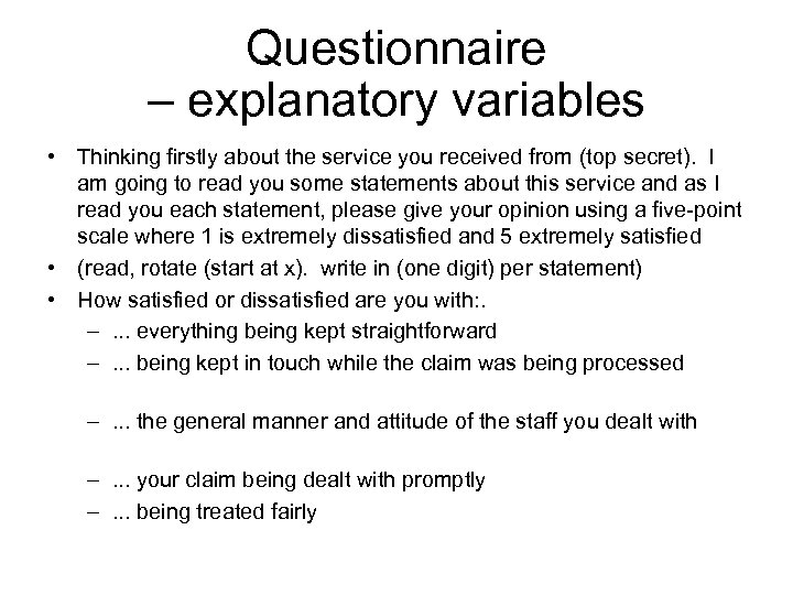Questionnaire – explanatory variables • Thinking firstly about the service you received from (top secret). I am going to read you some statements about this service and as I read you each statement, please give your opinion using a five-point scale where 1 is extremely dissatisfied and 5 extremely satisfied • (read, rotate (start at x). write in (one digit) per statement) • How satisfied or dissatisfied are you with: . –. . . everything being kept straightforward –. . . being kept in touch while the claim was being processed –. . . the general manner and attitude of the staff you dealt with –. . . your claim being dealt with promptly –. . . being treated fairly

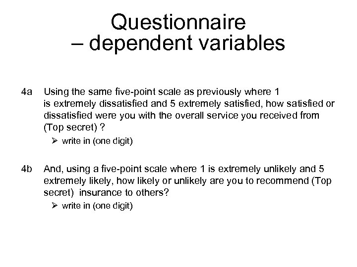Questionnaire – dependent variables 4 a Using the same five-point scale as previously where 1 is extremely dissatisfied and 5 extremely satisfied, how satisfied or dissatisfied were you with the overall service you received from (Top secret) ? Ø write in (one digit) 4 b And, using a five-point scale where 1 is extremely unlikely and 5 extremely likely, how likely or unlikely are you to recommend (Top secret) insurance to others? Ø write in (one digit)

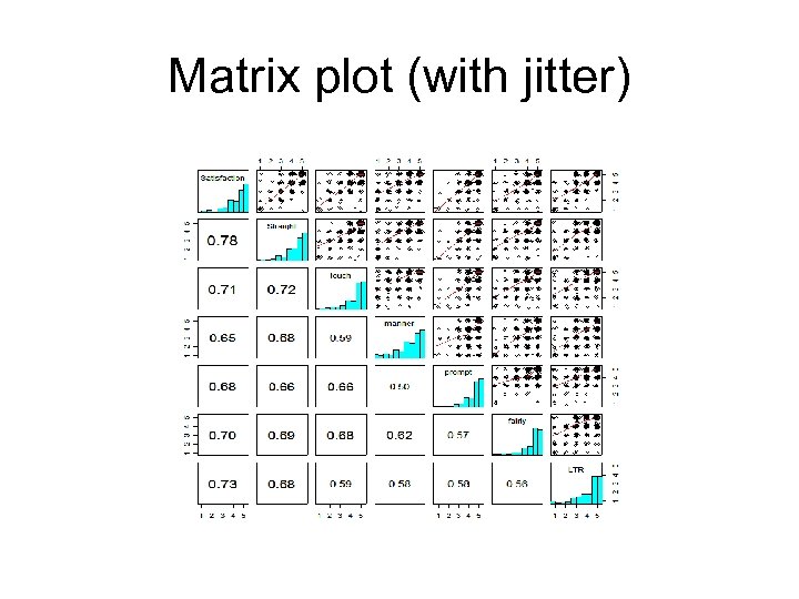Matrix plot (with jitter)

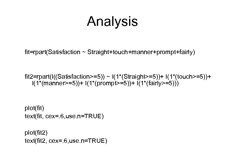Analysis fit=rpart(Satisfaction ~ Straight+touch+manner+prompt+fairly) fit 2=rpart(I((Satisfaction>=5)) ~ I(1*(Straight>=5))+ I(1*(touch>=5))+ I(1*(manner>=5))+ I(1*(prompt>=5))+ I(1*(fairly>=5))) plot(fit) text(fit, cex=. 6, use. n=TRUE) plot(fit 2) text(fit 2, cex=. 6, use. n=TRUE)

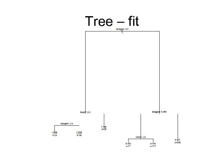Tree – fit

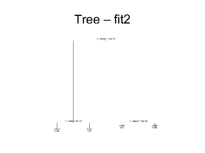Tree – fit 2

Cross-Validation • Due to over-fitting, cannot estimate prediction error directly on the training dataset • Cross-validation is a simple and widely used method for estimating prediction error • Simple approach – Set aside a test dataset – Train learner on the remainder (the training dataset) – Estimate prediction error by using the resulting prediction model on the test dataset • This is only feasible where there is enough data to set aside a test dataset and still have enough to reliably train the learning algorithm

Regression Example –revisited (yet again) samp=sample(1: nrow(ASB), round(. 8*nrow(ASB), 0), replace=FALSE) ASB. train=ASB[samp, ] ASB. test=ASB[-samp, ] fit 3=rpart(I((Satisfaction>=5)) ~ I(1*(Straight>=5))+ I(1*(touch>=5))+ I(1*(manner>=5))+ I(1*(prompt>=5))+ I(1*(fairly>=5)), data=ASB. train) obs=1*(ASB. test[, "Satisfaction"]>=5) pred=1*(predict(fit 3, ASB. test)>. 5) Pred. ASB<-matrix(c( sum(obs==0&pred==0), sum(obs==0&pred==1), sum(obs==1&pred==0), sum(obs==1&pred==1)), byrow=T, 2, 2) dimnames(Pred. ASB)=list(c("Obs<5", "Obs>=5"), c(" Pred<5", "Pred>=5")) Pred<5 Pred>=5 Obs<5 41 11 Obs>=5 10 47 > sum(diag(Pred. ASB))/sum(Pred. ASB) [1] 0. 8073394

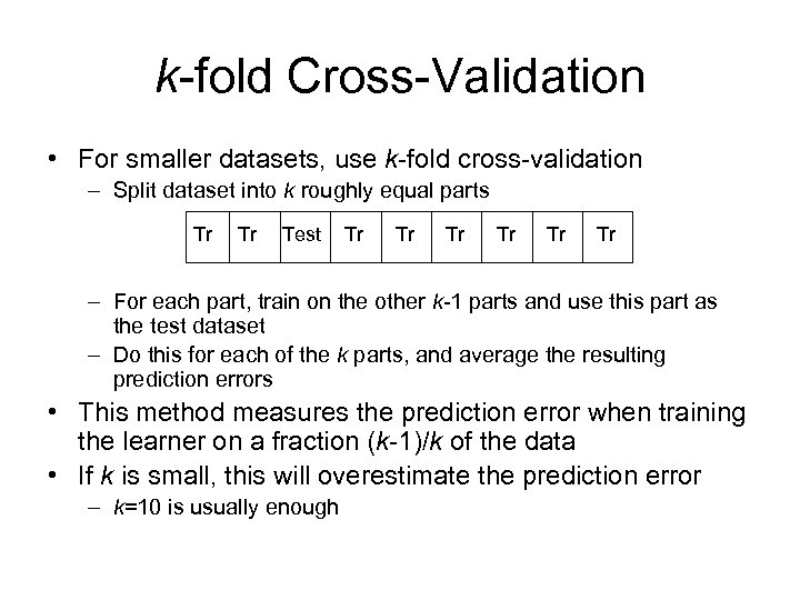k-fold Cross-Validation • For smaller datasets, use k-fold cross-validation – Split dataset into k roughly equal parts Tr Tr Test Tr Tr Tr – For each part, train on the other k-1 parts and use this part as the test dataset – Do this for each of the k parts, and average the resulting prediction errors • This method measures the prediction error when training the learner on a fraction (k-1)/k of the data • If k is small, this will overestimate the prediction error – k=10 is usually enough

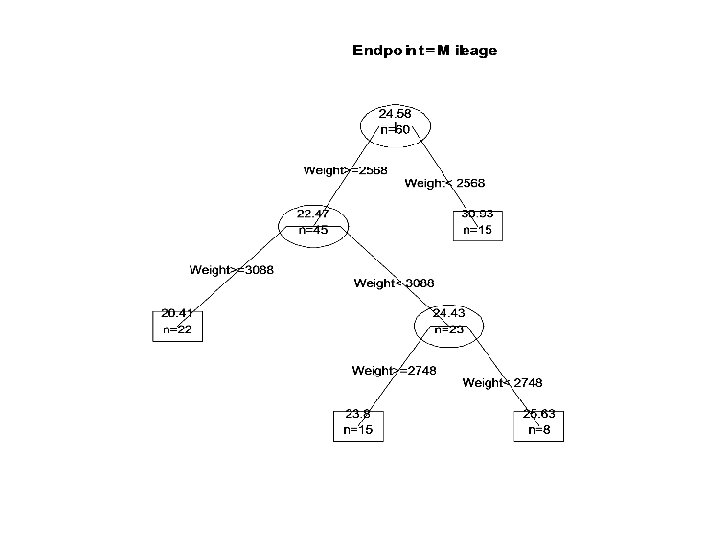
Regression Tree Example • data(car. test. frame) • z. auto <- rpart(Mileage ~ Weight, car. test. frame) • post(z. auto, file=“”) • summary(z. auto)

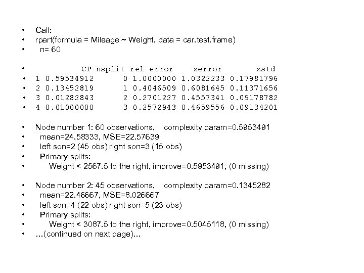• • • Call: rpart(formula = Mileage ~ Weight, data = car. test. frame) n= 60 • • • 1 2 3 4 • • • Node number 1: 60 observations, complexity param=0. 5953491 mean=24. 58333, MSE=22. 57639 left son=2 (45 obs) right son=3 (15 obs) Primary splits: Weight < 2567. 5 to the right, improve=0. 5953491, (0 missing) • • • Node number 2: 45 observations, complexity param=0. 1345282 mean=22. 46667, MSE=8. 026667 left son=4 (22 obs) right son=5 (23 obs) Primary splits: Weight < 3087. 5 to the right, improve=0. 5045118, (0 missing) …(continued on next page)… CP nsplit rel error 0. 59534912 0 1. 0000000 0. 13452819 1 0. 4046509 0. 01282843 2 0. 2701227 0. 01000000 3 0. 2572943 xerror 1. 0322233 0. 6081645 0. 4557341 0. 4659556 xstd 0. 17981796 0. 11371656 0. 09178782 0. 09134201

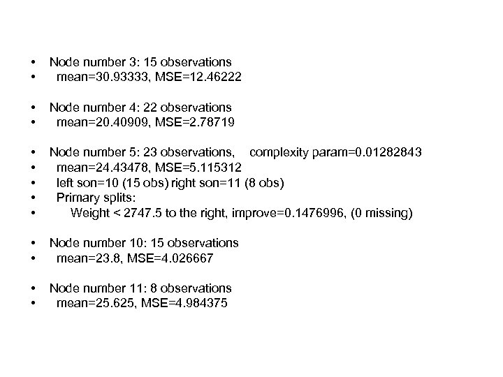• • Node number 3: 15 observations mean=30. 93333, MSE=12. 46222 • • Node number 4: 22 observations mean=20. 40909, MSE=2. 78719 • • • Node number 5: 23 observations, complexity param=0. 01282843 mean=24. 43478, MSE=5. 115312 left son=10 (15 obs) right son=11 (8 obs) Primary splits: Weight < 2747. 5 to the right, improve=0. 1476996, (0 missing) • • Node number 10: 15 observations mean=23. 8, MSE=4. 026667 • • Node number 11: 8 observations mean=25. 625, MSE=4. 984375

Regression Tree Example (continued) • plotcp(z. auto) • z 2. auto <- prune(z. auto, cp=0. 1) • post(z 2. auto, file="", cex=1)

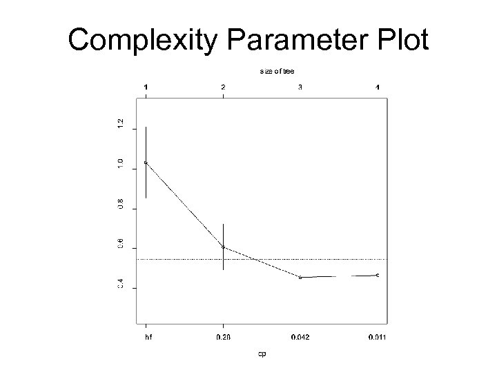Complexity Parameter Plot

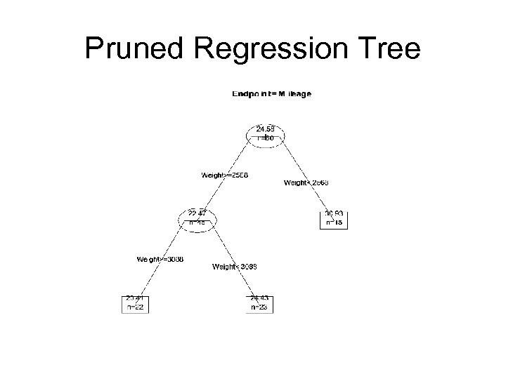Pruned Regression Tree

Classification Methods • Project the attribute space into decision regions – Decision trees: piecewise constant approximation – Logistic regression: linear log-odds approximation – Discriminant analysis and neural nets: linear & non-linear separators • Density estimation coupled with a decision rule – E. g. Naïve Bayes • Define a metric space and decide based on proximity – One type of instance-based learning – K-nearest neighbour methods • IBk algorithm in Weka – Would like to drop noisy and unnecessary points • Simple algorithm based on success rate confidence intervals available in Weka – Compares naïve prediction with predictions using that instance – Must choose suitable acceptance and rejection confidence levels • Many of these approaches can produce probability distributions as well as predictions – Depending on the application, this information may be useful • Such as when results reported to expert (e. g. loan officer) as input to their decision

Numeric Prediction Methods • Linear regression • Splines, including smoothing splines and multivariate adaptive regression splines (MARS) • Generalised additive models (GAM) • Locally weighted regression (lowess, loess) • Regression and Model Trees – CART, C 4. 5, M 5’ • Artificial neural networks (ANNs)

Artificial Neural Networks (ANNs) • An ANN is a network of many simple processors (or units), that are connected by communication channels that carry numeric data • ANNs are very flexible, encompassing nonlinear regression models, discriminant models, and data reduction models – They do require some expertise to set up – An appropriate architecture needs to be selected and tuned for each application • They can be useful tools for learning from examples to find patterns in data and predict outputs – However on their own, they tend to overfit the training data – Meta-learning tools are needed to choose the best fit • Various network architectures in common use – Multilayer perceptron (MLR) – Radial basis functions (RBF) – Self-organising maps (SOM) • ANNs have been applied to data editing and imputation, but not widely

Meta-Learning Methods - Bagging • General methods for improving the performance of most learning algorithms • Bootstrap aggregation, bagging for short – Select B bootstrap samples from the data • Selected with replacement, same # of instances – Can use parametric or non-parametric bootstrap – Fit the model/learner on each bootstrap sample – The bagged estimate is the average prediction from all these B models • E. g. for a tree learner, the bagged estimate is the average prediction from the resulting B trees • Note that this is not a tree – In general, bagging a model or learner does not produce a model or learner of the same form • Bagging reduces the variance of unstable procedures like regression trees, and can greatly improve prediction accuracy – However it does not always work for poor 0 -1 predictors

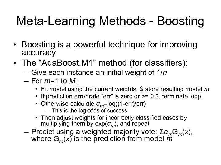Meta-Learning Methods - Boosting • Boosting is a powerful technique for improving accuracy • The “Ada. Boost. M 1” method (for classifiers): – Give each instance an initial weight of 1/n – For m=1 to M: • Fit model using the current weights, & store resulting model m • If prediction error rate “err” is zero or >= 0. 5, terminate loop. • Otherwise calculate αm=log((1 -err)/err) – This is the log odds of success • Then adjust weights for incorrectly classified cases by multiplying them by exp(αm), and repeat – Predict using a weighted majority vote: Σαm. Gm(x), where Gm(x) is the prediction from model m

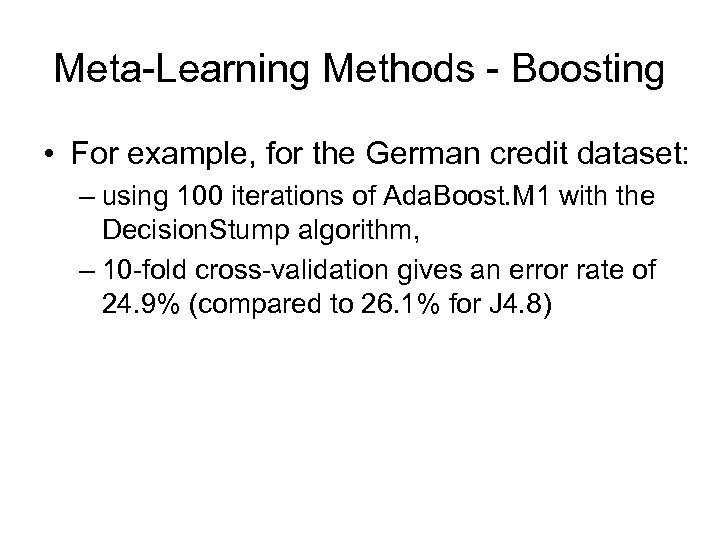Meta-Learning Methods - Boosting • For example, for the German credit dataset: – using 100 iterations of Ada. Boost. M 1 with the Decision. Stump algorithm, – 10 -fold cross-validation gives an error rate of 24. 9% (compared to 26. 1% for J 4. 8)

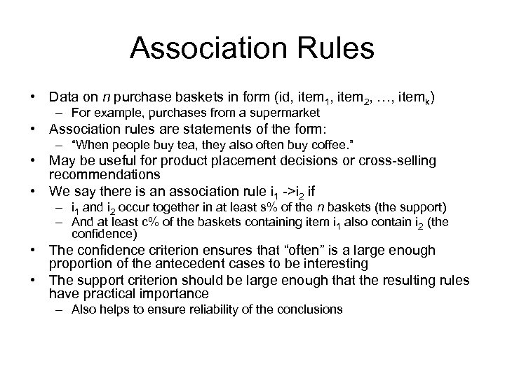Association Rules • Data on n purchase baskets in form (id, item 1, item 2, …, itemk) – For example, purchases from a supermarket • Association rules are statements of the form: – “When people buy tea, they also often buy coffee. ” • May be useful for product placement decisions or cross-selling recommendations • We say there is an association rule i 1 ->i 2 if – i 1 and i 2 occur together in at least s% of the n baskets (the support) – And at least c% of the baskets containing item i 1 also contain i 2 (the confidence) • The confidence criterion ensures that “often” is a large enough proportion of the antecedent cases to be interesting • The support criterion should be large enough that the resulting rules have practical importance – Also helps to ensure reliability of the conclusions

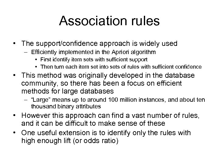Association rules • The support/confidence approach is widely used – Efficiently implemented in the Apriori algorithm • First identify item sets with sufficient support • Then turn each item set into sets of rules with sufficient confidence • This method was originally developed in the database community, so there has been a focus on efficient methods for large databases – “Large” means up to around 100 million instances, and about ten thousand binary attributes • However this approach can find a vast number of rules, and it can be difficult to make sense of these • One useful extension is to identify only the rules with high enough lift (or odds ratio)

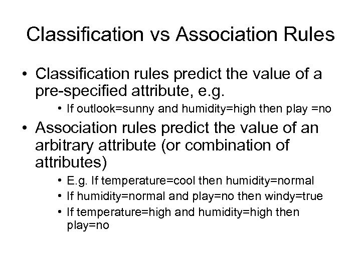Classification vs Association Rules • Classification rules predict the value of a pre-specified attribute, e. g. • If outlook=sunny and humidity=high then play =no • Association rules predict the value of an arbitrary attribute (or combination of attributes) • E. g. If temperature=cool then humidity=normal • If humidity=normal and play=no then windy=true • If temperature=high and humidity=high then play=no

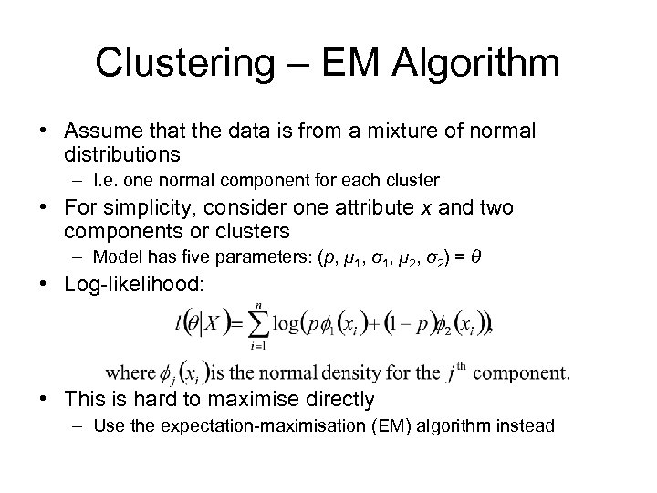Clustering – EM Algorithm • Assume that the data is from a mixture of normal distributions – I. e. one normal component for each cluster • For simplicity, consider one attribute x and two components or clusters – Model has five parameters: (p, μ 1, σ1, μ 2, σ2) = θ • Log-likelihood: • This is hard to maximise directly – Use the expectation-maximisation (EM) algorithm instead

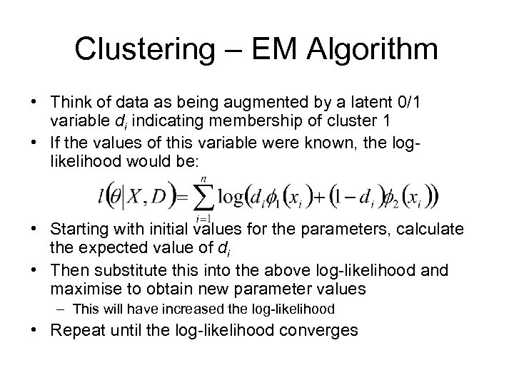Clustering – EM Algorithm • Think of data as being augmented by a latent 0/1 variable di indicating membership of cluster 1 • If the values of this variable were known, the loglikelihood would be: • Starting with initial values for the parameters, calculate the expected value of di • Then substitute this into the above log-likelihood and maximise to obtain new parameter values – This will have increased the log-likelihood • Repeat until the log-likelihood converges

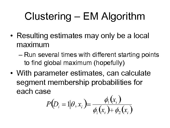Clustering – EM Algorithm • Resulting estimates may only be a local maximum – Run several times with different starting points to find global maximum (hopefully) • With parameter estimates, can calculate segment membership probabilities for each case

Clustering – EM Algorithm • Extending to more latent classes is easy – Information criteria such as AIC and BIC are often used to decide how many are appropriate • Extending to multiple attributes is easy if we assume they are independent, at least conditioning on segment membership – It is possible to introduce associations, but this can rapidly increase the number of parameters required • Nominal attributes can be accommodated by allowing different discrete distributions in each latent class, and assuming conditional independence between attributes • Can extend this approach to a handle joint clustering and prediction models, as mentioned in the MVA lectures

Clustering - Scalability Issues • • • k-means algorithm is also widely used However this and the EM-algorithm are slow on large databases So is hierarchical clustering - requires O(n 2) time Iterative clustering methods require full DB scan at each iteration Scalable clustering algorithms are an area of active research A few recent algorithms: – Distance-based/k-Means • • Multi-Resolution kd-Tree for K-Means [PM 99] CLIQUE [AGGR 98] Scalable K-Means [BFR 98 a] CLARANS [NH 94] – Probabilistic/EM • Multi-Resolution kd-Tree for EM [Moore 99] • Scalable EM [BRF 98 b] • CF Kernel Density Estimation [ZRL 99]

Ethics of Data Mining • Data mining and data warehousing raise ethical and legal issues • Combining information via data warehousing could violate Privacy Act – Must tell people how their information will be used when the data is obtained • Data mining raises ethical issues mainly during application of results – E. g. using ethnicity as a factor in loan approval decisions – E. g. screening job applications based on age or sex (where not directly relevant) – E. g. declining insurance coverage based on neighbourhood if this is related to race (“red-lining” is illegal in much of the US) • Whether something is ethical depends on the application – E. g. probably ethical to use ethnicity to diagnose and choose treatments for a medical problem, but not to decline medical insurance