27828c88d66e4f6a9649297548c067f7.ppt
- Количество слайдов: 27
Data Mining Copyright: Silberschatz, Korth and Sudarshan 1
Data Mining n Broadly speaking, data mining is the process of semi- automatically analyzing large databases to find useful patterns n Like knowledge discovery in artificial intelligence data mining discovers statistical rules and patterns n Differs from machine learning in that it deals with large volumes of data stored primarily on disk. n Some types of knowledge discovered from a database can be represented by a set of rules. H e. g. , : “Young women with annual incomes greater than $50, 000 are most likely to buy sports cars” n Other types of knowledge represented by equations, or by prediction functions n Some manual intervention is usually required H Pre-processing of data, choice of which type of pattern to find, postprocessing to find novel patterns 2 Database System Concepts 4 th Edition 22. 2 ©Silberschatz, Korth and Sudarshan
Applications of Data Mining n Prediction based on past history H Predict if a credit card applicant poses a good credit risk, based on some attributes (income, job type, age, . . ) and past history H Predict if a customer is likely to switch brand loyalty H Predict if a customer is likely to respond to “junk mail” H Predict if a pattern of phone calling card usage is likely to be fraudulent n Some examples of prediction mechanisms: H Classification 4 Given a training set consisting of items belonging to different classes, and a new item whose class is unknown, predict which class it belongs to H Regression formulae 4 given a set of parameter-value to function-result mappings for an unknown function, predict the function-result for a new parameter -value 3 Database System Concepts 4 th Edition 22. 3 ©Silberschatz, Korth and Sudarshan
Applications of Data Mining (Cont. ) n Descriptive Patterns H Associations 4 Find books that are often bought by the same customers. If a new customer buys one such book, suggest that he buys the others too. 4 Other similar applications: camera accessories, clothes, etc. H Associations may also be used as a first step in detecting causation 4 E. g. association between exposure to chemical X and cancer, or new medicine and cardiac problems H Clusters 4 E. g. typhoid cases were clustered in an area surrounding a contaminated well 4 Detection of clusters remains important in detecting epidemics 4 Database System Concepts 4 th Edition 22. 4 ©Silberschatz, Korth and Sudarshan
Classification Rules n Classification rules help assign new objects to a set of classes. E. g. , given a new automobile insurance applicant, should he or she be classified as low risk, medium risk or high risk? n Classification rules for above example could use a variety of knowledge, such as educational level of applicant, salary of applicant, age of applicant, etc. H person P, P. degree = masters and P. income > 75, 000 P. credit = excellent H person P, P. degree = bachelors and (P. income 25, 000 and P. income 75, 000) P. credit = good n Rules are not necessarily exact: there may be some misclassifications n Classification rules can be compactly shown as a decision tree. 5 Database System Concepts 4 th Edition 22. 5 ©Silberschatz, Korth and Sudarshan
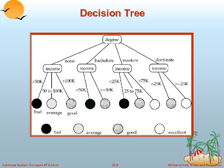
Decision Tree 6 Database System Concepts 4 th Edition 22. 6 ©Silberschatz, Korth and Sudarshan
Construction of Decision Trees n Training set: a data sample in which the grouping for each tuple is already known. n Consider credit risk example: Suppose degree is chosen to partition the data at the root. H Since degree has a small number of possible values, one child is created for each value. n At each child node of the root, further classification is done if required. Here, partitions are defined by income. H Since income is a continuous attribute, some number of intervals are chosen, and one child created for each interval. n Different classification algorithms use different ways of choosing which attribute to partition on at each node, and what the intervals, if any, are. n In general H Different branches of the tree could grow to different levels. H Different nodes at the same level may use different partitioning attributes. 7 Database System Concepts 4 th Edition 22. 7 ©Silberschatz, Korth and Sudarshan
Construction of Decision Trees (Cont. ) n Greedy top down generation of decision trees. H Each internal node of the tree partitions the data into groups based on a partitioning attribute, and a partitioning condition for the node 4 More on choosing partioning attribute/condition shortly 4 Algorithm is greedy: the choice is made once and not revisited as more of the tree is constructed H The data at a node is not partitioned further if either 4 all (or most) of the items at the node belong to the same class, or 4 all attributes have been considered, and no further partitioning is possible. Such a node is a leaf node. H Otherwise the data at the node is partitioned further by picking an attribute for partitioning data at the node. 8 Database System Concepts 4 th Edition 22. 8 ©Silberschatz, Korth and Sudarshan
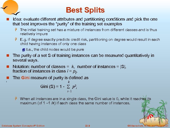
Best Splits n Idea: evaluate different attributes and partitioning conditions and pick the one that best improves the “purity” of the training set examples H The initial training set has a mixture of instances from different classes and is thus relatively impure H E. g. if degree exactly predicts credit risk, partitioning on degree would result in each child having instances of only one class 4 I. e. , the child nodes would be pure n The purity of a set S of training instances can be measured quantitatively in several ways. n Notation: number of classes = k, number of instances = |S|, fraction of instances in class i = pi. n The Gini measure of purity is defined as k [ Gini (S) = 1 - p 2 i i- 1 H When all instances are in a single class, the Gini value is 0, while it reaches its maximum (of 1 – 1 /k) if each class the same number of instances. 9 Database System Concepts 4 th Edition 22. 9 ©Silberschatz, Korth and Sudarshan
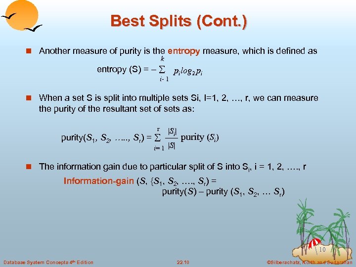
Best Splits (Cont. ) n Another measure of purity is the entropy measure, which is defined as k entropy (S) = – i- 1 pilog 2 pi n When a set S is split into multiple sets Si, I=1, 2, …, r, we can measure the purity of the resultant set of sets as: r purity(S 1, S 2, …. . , Sr) = |Si| i= 1 |S| purity (Si) n The information gain due to particular split of S into Si, i = 1, 2, …. , r Information-gain (S, {S 1, S 2, …. , Sr) = purity(S) – purity (S 1, S 2, … Sr) 10 Database System Concepts 4 th Edition 22. 10 ©Silberschatz, Korth and Sudarshan
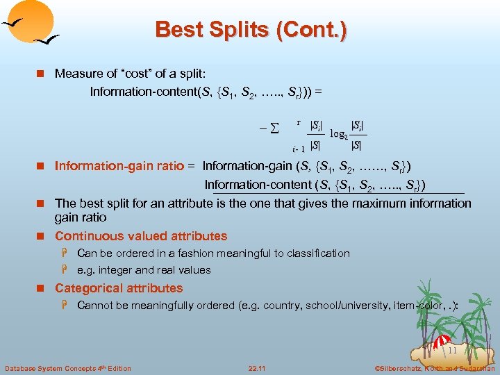
Best Splits (Cont. ) n Measure of “cost” of a split: Information-content(S, {S 1, S 2, …. . , Sr})) = – r |S | i i- 1 |S| log 2 |Si| |S| n Information-gain ratio = Information-gain (S, {S 1, S 2, ……, Sr}) Information-content (S, {S 1, S 2, …. . , Sr}) n The best split for an attribute is the one that gives the maximum information gain ratio n Continuous valued attributes H Can be ordered in a fashion meaningful to classification H e. g. integer and real values n Categorical attributes H Cannot be meaningfully ordered (e. g. country, school/university, item-color, . ): 11 Database System Concepts 4 th Edition 22. 11 ©Silberschatz, Korth and Sudarshan
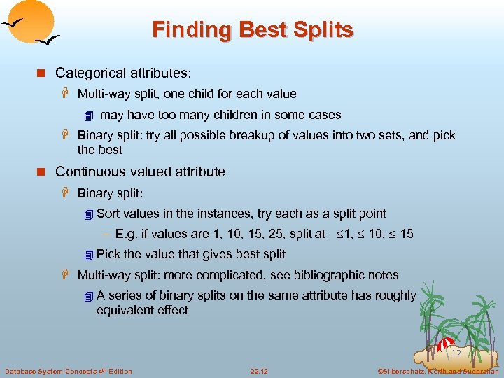
Finding Best Splits n Categorical attributes: H Multi-way split, one child for each value 4 may have too many children in some cases H Binary split: try all possible breakup of values into two sets, and pick the best n Continuous valued attribute H Binary split: 4 Sort values in the instances, try each as a split point – E. g. if values are 1, 10, 15, 25, split at 1, 10, 15 4 Pick the value that gives best split H Multi-way split: more complicated, see bibliographic notes 4 A series of binary splits on the same attribute has roughly equivalent effect 12 Database System Concepts 4 th Edition 22. 12 ©Silberschatz, Korth and Sudarshan
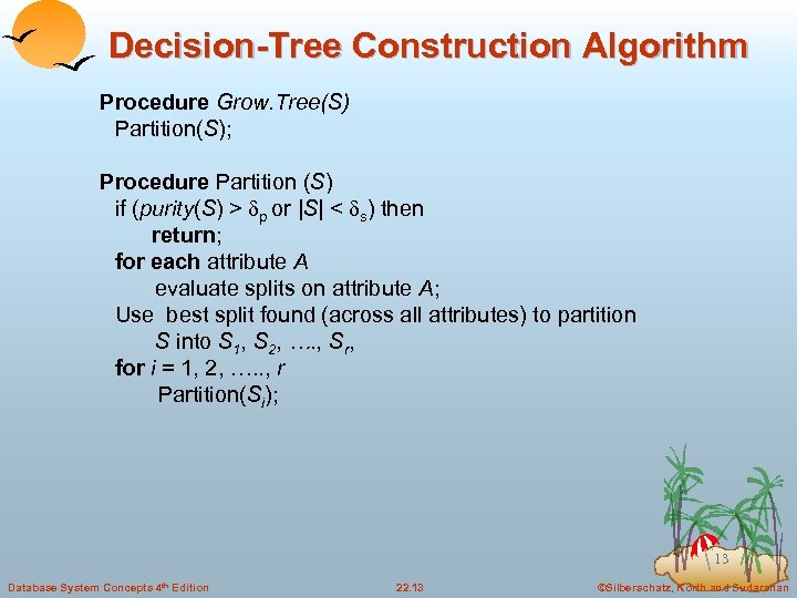
Decision-Tree Construction Algorithm Procedure Grow. Tree(S) Partition(S); Procedure Partition (S) if (purity(S) > p or |S| < s) then return; for each attribute A evaluate splits on attribute A; Use best split found (across all attributes) to partition S into S 1, S 2, …. , Sr, for i = 1, 2, …. . , r Partition(Si); 13 Database System Concepts 4 th Edition 22. 13 ©Silberschatz, Korth and Sudarshan
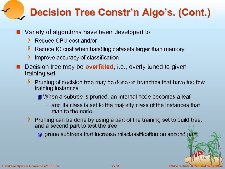
Decision Tree Constr’n Algo’s. (Cont. ) n Variety of algorithms have been developed to H Reduce CPU cost and/or H Reduce IO cost when handling datasets larger than memory H Improve accuracy of classification n Decision tree may be overfitted, i. e. , overly tuned to given training set H Pruning of decision tree may be done on branches that have too few training instances 4 When a subtree is pruned, an internal node becomes a leaf – and its class is set to the majority class of the instances that map to the node H Pruning can be done by using a part of the training set to build tree, and a second part to test the tree 4 prune subtrees that increase misclassification on second part 14 Database System Concepts 4 th Edition 22. 14 ©Silberschatz, Korth and Sudarshan
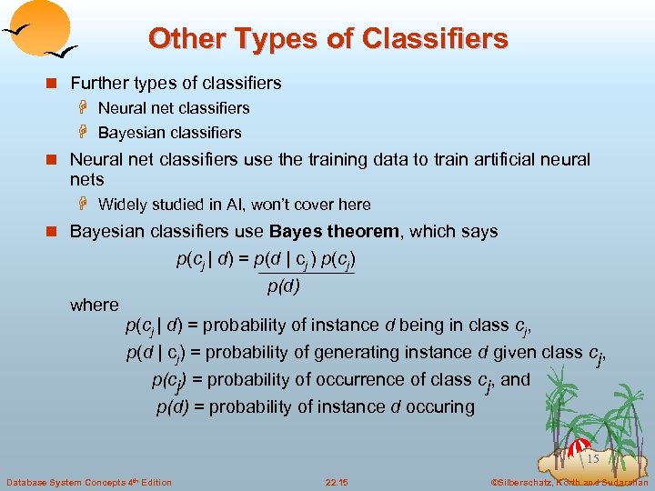
Other Types of Classifiers n Further types of classifiers H Neural net classifiers H Bayesian classifiers n Neural net classifiers use the training data to train artificial neural nets H Widely studied in AI, won’t cover here n Bayesian classifiers use Bayes theorem, which says p(cj | d) = p(d | cj ) p(cj) p(d) where p(cj | d) = probability of instance d being in class cj, p(d | cj) = probability of generating instance d given class cj, p(cj) = probability of occurrence of class cj, and p(d) = probability of instance d occuring 15 Database System Concepts 4 th Edition 22. 15 ©Silberschatz, Korth and Sudarshan
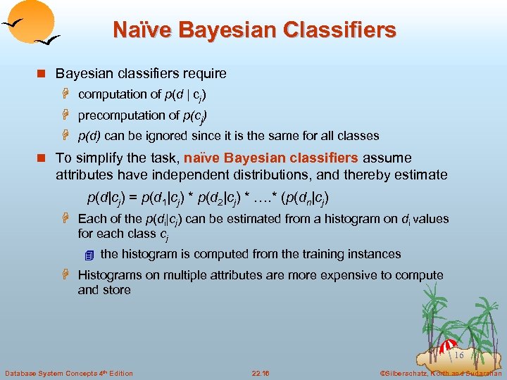
Naïve Bayesian Classifiers n Bayesian classifiers require H computation of p(d | cj) H precomputation of p(cj) H p(d) can be ignored since it is the same for all classes n To simplify the task, naïve Bayesian classifiers assume attributes have independent distributions, and thereby estimate p(d|cj) = p(d 1|cj) * p(d 2|cj) * …. * (p(dn|cj) H Each of the p(di|cj) can be estimated from a histogram on di values for each class cj 4 the histogram is computed from the training instances H Histograms on multiple attributes are more expensive to compute and store 16 Database System Concepts 4 th Edition 22. 16 ©Silberschatz, Korth and Sudarshan
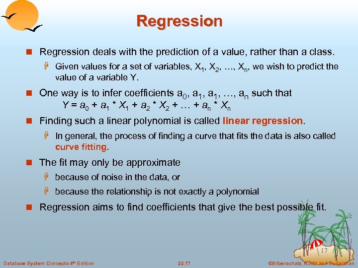
Regression n Regression deals with the prediction of a value, rather than a class. H Given values for a set of variables, X 1, X 2, …, Xn, we wish to predict the value of a variable Y. n One way is to infer coefficients a 0, a 1, …, an such that Y = a 0 + a 1 * X 1 + a 2 * X 2 + … + an * X n n Finding such a linear polynomial is called linear regression. H In general, the process of finding a curve that fits the data is also called curve fitting. n The fit may only be approximate H because of noise in the data, or H because the relationship is not exactly a polynomial n Regression aims to find coefficients that give the best possible fit. 17 Database System Concepts 4 th Edition 22. 17 ©Silberschatz, Korth and Sudarshan
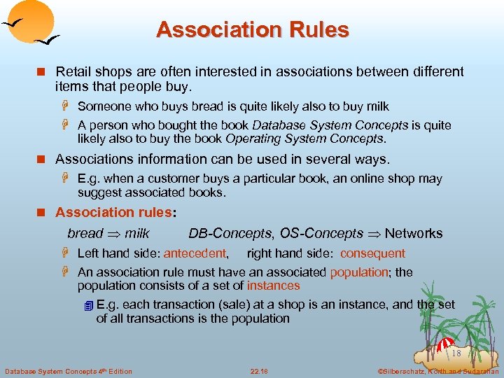
Association Rules n Retail shops are often interested in associations between different items that people buy. H Someone who buys bread is quite likely also to buy milk H A person who bought the book Database System Concepts is quite likely also to buy the book Operating System Concepts. n Associations information can be used in several ways. H E. g. when a customer buys a particular book, an online shop may suggest associated books. n Association rules: bread milk DB-Concepts, OS-Concepts Networks H Left hand side: antecedent, right hand side: consequent H An association rule must have an associated population; the population consists of a set of instances 4 E. g. each transaction (sale) at a shop is an instance, and the set of all transactions is the population 18 Database System Concepts 4 th Edition 22. 18 ©Silberschatz, Korth and Sudarshan
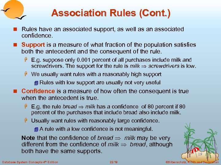
Association Rules (Cont. ) n Rules have an associated support, as well as an associated confidence. n Support is a measure of what fraction of the population satisfies both the antecedent and the consequent of the rule. H E. g. suppose only 0. 001 percent of all purchases include milk and screwdrivers. The support for the rule is milk screwdrivers is low. H We usually want rules with a reasonably high support 4 Rules with low support are usually not very useful n Confidence is a measure of how often the consequent is true when the antecedent is true. H E. g. the rule bread milk has a confidence of 80 percent if 80 percent of the purchases that include bread also include milk. H Usually want rules with reasonably large confidence. 4 A rule with a low confidence is not meaningful. Note that the confidence of bread milk may be very different from the confidence of milk bread, although both have the same supports. Database System Concepts 4 th Edition 22. 19 19 ©Silberschatz, Korth and Sudarshan
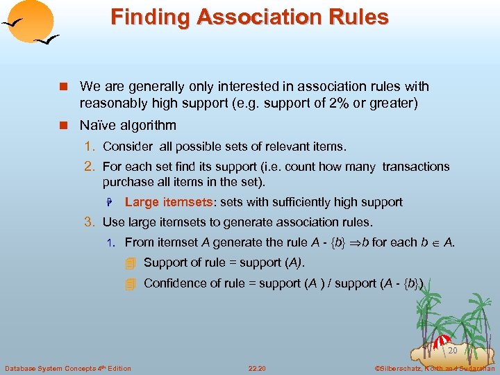
Finding Association Rules n We are generally only interested in association rules with reasonably high support (e. g. support of 2% or greater) n Naïve algorithm 1. Consider all possible sets of relevant items. 2. For each set find its support (i. e. count how many transactions purchase all items in the set). H Large itemsets: sets with sufficiently high support 3. Use large itemsets to generate association rules. 1. From itemset A generate the rule A - {b} b for each b A. 4 Support of rule = support (A). 4 Confidence of rule = support (A ) / support (A - {b}) 20 Database System Concepts 4 th Edition 22. 20 ©Silberschatz, Korth and Sudarshan
Finding Support n Few itemsets: determine support of all itemsets via a single pass on set of transactions H A count is maintained for each itemset, initially set to 0. H When a transaction is fetched, the count is incremented for each set of items that is contained in the transaction. H Large itemsets: sets with a high count at the end of the pass n Many itemsets: If memory not enough to hold all counts for all itemsets use multiple passes, considering only some itemsets in each pass. n Optimization: Once an itemset is eliminated because its count (support) is too small none of its supersets needs to be considered. n The a priori technique to find large itemsets: H Pass 1: count support of all sets with just 1 item. Eliminate those items with low support H Pass i: candidates: every set of i items such that all its i-1 item subsets are large 4 Count support of all candidates 4 Stop if there are no candidates 21 Database System Concepts 4 th Edition 22. 21 ©Silberschatz, Korth and Sudarshan
Other Types of Associations n Basic association rules have several limitations n Deviations from the expected probability are more interesting H E. g. if many people purchase bread, and many people purchase cereal, quite a few would be expected to purchase both (prob 1 * prob 2) H We are interested in positive as well as negative correlations between sets of items 4 Positive correlation: co-occurrence is higher than predicted 4 Negative correlation: co-occurrence is lower than predicted n Sequence associations/correlations H E. g. whenever bonds go up, stock prices go down in 2 days n Deviations from temporal patterns H E. g. deviation from a steady growth H E. g. sales of winter wear go down in summer 4 Not surprising, part of a known pattern. 4 Look for deviation from value predicted using past patterns 22 Database System Concepts 4 th Edition 22. 22 ©Silberschatz, Korth and Sudarshan
Clustering n Clustering: Intuitively, finding clusters of points in the given data such that similar points lie in the same cluster n Can be formalized using distance metrics in several ways n E. g. Group points into k sets (for a given k) such that the average distance of points from the centroid of their assigned group is minimized H Centroid: point defined by taking average of coordinates in each dimension. H Another metric: minimize average distance between every pair of points in a cluster n Has been studied extensively in statistics, but on small data sets H Data mining systems aim at clustering techniques that can handle very large data sets H E. g. the Birch clustering algorithm (more shortly) 23 Database System Concepts 4 th Edition 22. 23 ©Silberschatz, Korth and Sudarshan
Hierarchical Clustering n Example from biological classification H (the word classification here does not mean a prediction mechanism) chordata mammalia leopards humans reptilia snakes crocodiles n Other examples: Internet directory systems (e. g. Yahoo, more on this later) n Agglomerative clustering algorithms H Build small clusters, then cluster small clusters into bigger clusters, and so on n Divisive clustering algorithms H Start with all items in a single cluster, repeatedly refine (break) clusters into smaller ones 24 Database System Concepts 4 th Edition 22. 24 ©Silberschatz, Korth and Sudarshan
Clustering Algorithms n Clustering algorithms have been designed to handle very large datasets n E. g. the Birch algorithm H Main idea: use an in-memory R-tree to store points that are being clustered H Insert points one at a time into the R-tree, merging a new point with an existing cluster if is less than some distance away H If there are more leaf nodes than fit in memory, merge existing clusters that are close to each other H At the end of first pass we get a large number of clusters at the leaves of the R-tree 4 Merge clusters to reduce the number of clusters 25 Database System Concepts 4 th Edition 22. 25 ©Silberschatz, Korth and Sudarshan
Collaborative Filtering n Goal: predict what movies/books/… a person may be interested in, on the basis of H Past preferences of the person H Other people with similar past preferences H The preferences of such people for a new movie/book/… n One approach based on repeated clustering H Cluster people on the basis of preferences for movies H Then cluster movies on the basis of being liked by the same clusters of people H Again cluster people based on their preferences for (the newly created clusters of) movies H Repeat above till equilibrium n Above problem is an instance of collaborative filtering, where users collaborate in the task of filtering information to find information of interest 26 Database System Concepts 4 th Edition 22. 26 ©Silberschatz, Korth and Sudarshan
Other Types of Mining n Text mining: application of data mining to textual documents H E. g. cluster Web pages to find related pages H E. g. cluster pages a user has visited to organize their visit history H E. g. classify Web pages automatically into a Web directory n Data visualization systems help users examine large volumes of data and detect patterns visually H E. g. maps, charts, and color-coding 4 E. g. locations with problems shown in red on a map H Can visually encode large amounts of information on a single screen H Humans are very good a detecting visual patterns 27 Database System Concepts 4 th Edition 22. 27 ©Silberschatz, Korth and Sudarshan
27828c88d66e4f6a9649297548c067f7.ppt