Data Mining Concepts and Techniques Slides for

Data Mining: Concepts and Techniques — Slides for Textbook — — Chapter 7 — ©Jiawei Han and Micheline Kamber Department of Computer Science University of Illinois at Urbana-Champaign www. cs. uiuc. edu/~hanj 1

Chapter 7. Classification and Prediction n n What is classification? What is prediction? Issues regarding classification and prediction Classification by decision tree induction Bayesian Classification by Neural Networks Classification by Support Vector Machines (SVM) Classification based on concepts from association rule mining Other Classification Methods Prediction Classification accuracy Summary 2

Bayesian Classification: Why? n n Probabilistic learning: Calculate explicit probabilities for hypothesis, among the most practical approaches to certain types of learning problems Incremental: Each training example can incrementally increase/decrease the probability that a hypothesis is correct. Prior knowledge can be combined with observed data. Probabilistic prediction: Predict multiple hypotheses, weighted by their probabilities Standard: Even when Bayesian methods are computationally intractable, they can provide a standard of optimal decision making against which other methods can be measured 3

Bayesian Theorem: Basics n n n Let X be a data sample whose class label is unknown Let H be a hypothesis that X belongs to class C For classification problems, determine P(H/X): the probability that the hypothesis holds given the observed data sample X P(H): prior probability of hypothesis H (i. e. the initial probability before we observe any data, reflects the background knowledge) P(X): probability that sample data is observed P(X|H) : probability of observing the sample X, given that the hypothesis holds 4

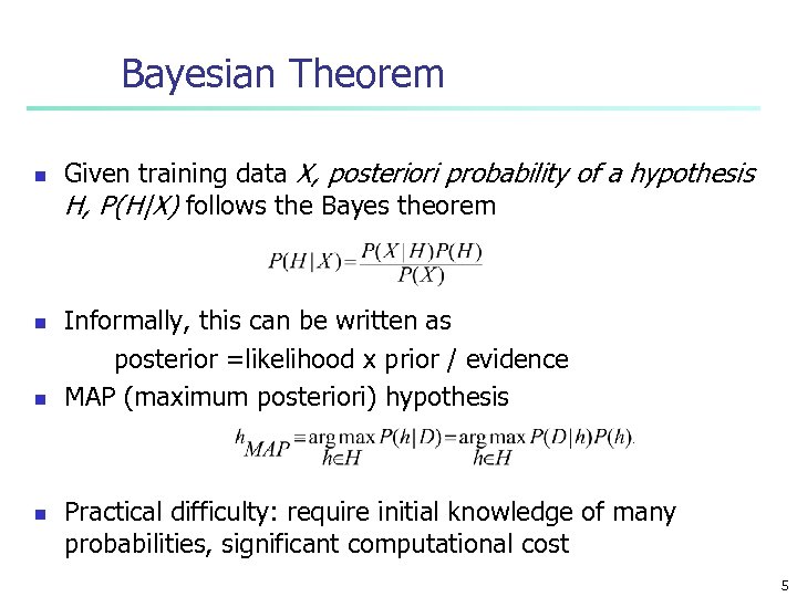Bayesian Theorem n n Given training data X, posteriori probability of a hypothesis H, P(H|X) follows the Bayes theorem Informally, this can be written as posterior =likelihood x prior / evidence MAP (maximum posteriori) hypothesis Practical difficulty: require initial knowledge of many probabilities, significant computational cost 5

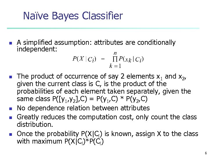Naïve Bayes Classifier n n n A simplified assumption: attributes are conditionally independent: The product of occurrence of say 2 elements x 1 and x 2, given the current class is C, is the product of the probabilities of each element taken separately, given the same class P([y 1, y 2], C) = P(y 1, C) * P(y 2, C) No dependence relation between attributes Greatly reduces the computation cost, only count the class distribution. Once the probability P(X|Ci) is known, assign X to the class with maximum P(X|Ci)*P(Ci) 6

Example n n n H X is an apple P(H) priori probability that X is an apple X observed data round and red P(H/X) probability that X is an apple given that we observe that it is red and round P(X/H) posteriori probability that a data is red and round given that it is an apple P(X) priori probabilility that it is red and round 7

Applying Bayesian Theorem n n n n P(H/X) = P(H, X)/P(X) from Bayesian theorem Similarly: P(X/H) = P(H, X)/P(H) P(H, X) = P(X/H)P(H) hence P(H/X) = P(X/H)P(H)/P(X) calculate P(H/X) from P(X/H), P(X) 8

Bayesian classification n n The classification problem may be formalized using a-posteriori probabilities: P(Ci|X) = prob. that the sample tuple X= is of class Ci. There are m classes Ci i =1 to m E. g. P(class=N | outlook=sunny, windy=true, …) Idea: assign to sample X the class label Ci such that P(Ci|X) is maximal P(Ci|X)> P(Cj|X) 1<=j<=m j i 11

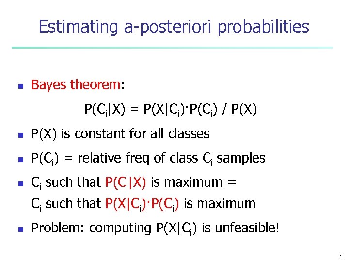Estimating a-posteriori probabilities n Bayes theorem: P(Ci|X) = P(X|Ci)·P(Ci) / P(X) n P(X) is constant for all classes n P(Ci) = relative freq of class Ci samples n Ci such that P(Ci|X) is maximum = Ci such that P(X|Ci)·P(Ci) is maximum n Problem: computing P(X|Ci) is unfeasible! 12

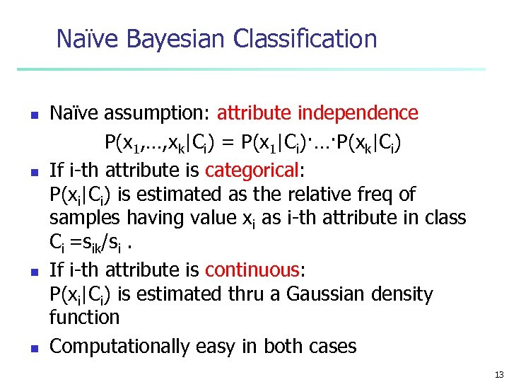Naïve Bayesian Classification n n Naïve assumption: attribute independence P(x 1, …, xk|Ci) = P(x 1|Ci)·…·P(xk|Ci) If i-th attribute is categorical: P(xi|Ci) is estimated as the relative freq of samples having value xi as i-th attribute in class Ci =sik/si. If i-th attribute is continuous: P(xi|Ci) is estimated thru a Gaussian density function Computationally easy in both cases 13

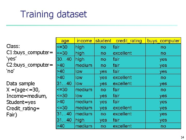Training dataset Class: C 1: buys_computer= ‘yes’ C 2: buys_computer= ‘no’ Data sample X =(age<=30, Income=medium, Student=yes Credit_rating= Fair) 14

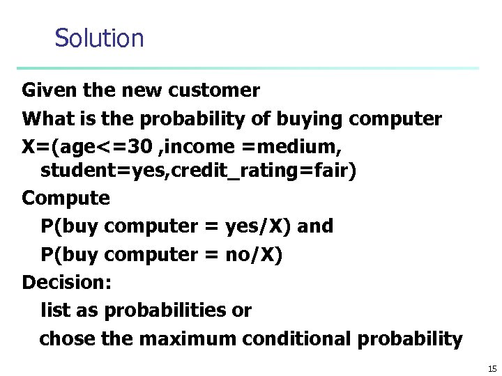Solution Given the new customer What is the probability of buying computer X=(age<=30 , income =medium, student=yes, credit_rating=fair) Compute P(buy computer = yes/X) and P(buy computer = no/X) Decision: list as probabilities or chose the maximum conditional probability 15

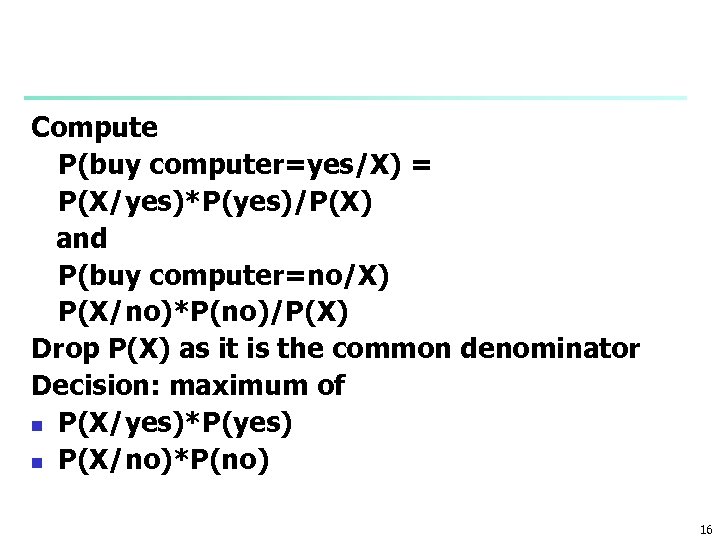Compute P(buy computer=yes/X) = P(X/yes)*P(yes)/P(X) and P(buy computer=no/X) P(X/no)*P(no)/P(X) Drop P(X) as it is the common denominator Decision: maximum of n P(X/yes)*P(yes) n P(X/no)*P(no) 16

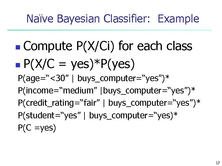Naïve Bayesian Classifier: Example Compute P(X/Ci) for each class n P(X/C = yes)*P(yes) n P(age=“<30” | buys_computer=“yes”)* P(income=“medium” |buys_computer=“yes”)* P(credit_rating=“fair” | buys_computer=“yes”)* P(student=“yes” | buys_computer=“yes)* P(C =yes) 17

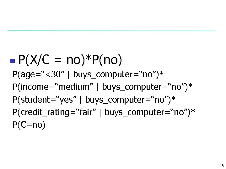n P(X/C = no)*P(no) P(age=“<30” | buys_computer=“no”)* P(income=“medium” | buys_computer=“no”)* P(student=“yes” | buys_computer=“no”)* P(credit_rating=“fair” | buys_computer=“no”)* P(C=no) 18

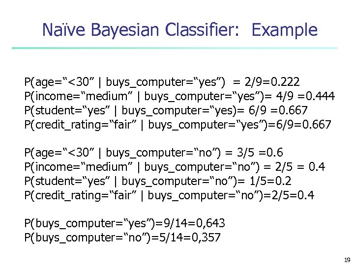Naïve Bayesian Classifier: Example P(age=“<30” | buys_computer=“yes”) = 2/9=0. 222 P(income=“medium” | buys_computer=“yes”)= 4/9 =0. 444 P(student=“yes” | buys_computer=“yes)= 6/9 =0. 667 P(credit_rating=“fair” | buys_computer=“yes”)=6/9=0. 667 P(age=“<30” | buys_computer=“no”) = 3/5 =0. 6 P(income=“medium” | buys_computer=“no”) = 2/5 = 0. 4 P(student=“yes” | buys_computer=“no”)= 1/5=0. 2 P(credit_rating=“fair” | buys_computer=“no”)=2/5=0. 4 P(buys_computer=“yes”)=9/14=0, 643 P(buys_computer=“no”)=5/14=0, 357 19

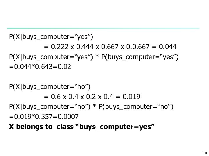P(X|buys_computer=“yes”) = 0. 222 x 0. 444 x 0. 667 x 0. 0. 667 = 0. 044 P(X|buys_computer=“yes”) * P(buys_computer=“yes”) =0. 044*0. 643=0. 02 P(X|buys_computer=“no”) = 0. 6 x 0. 4 x 0. 2 x 0. 4 = 0. 019 P(X|buys_computer=“no”) * P(buys_computer=“no”) =0. 019*0. 357=0. 0007 X belongs to class “buys_computer=yes” 20

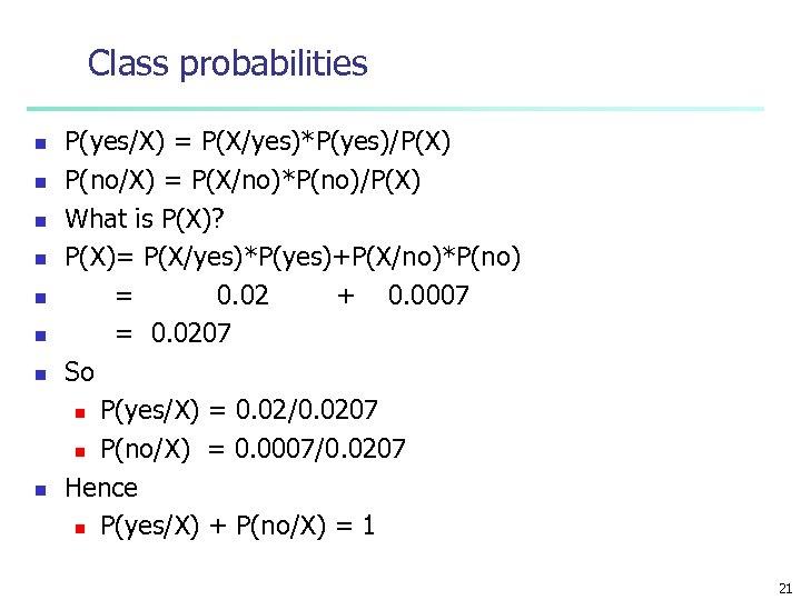Class probabilities n n n n P(yes/X) = P(X/yes)*P(yes)/P(X) P(no/X) = P(X/no)*P(no)/P(X) What is P(X)? P(X)= P(X/yes)*P(yes)+P(X/no)*P(no) = 0. 02 + 0. 0007 = 0. 0207 So n P(yes/X) = 0. 02/0. 0207 n P(no/X) = 0. 0007/0. 0207 Hence n P(yes/X) + P(no/X) = 1 21

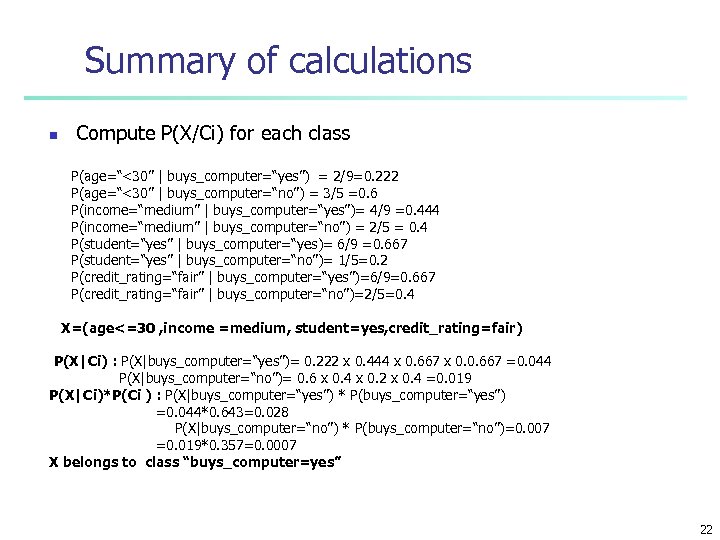Summary of calculations n Compute P(X/Ci) for each class P(age=“<30” | buys_computer=“yes”) = 2/9=0. 222 P(age=“<30” | buys_computer=“no”) = 3/5 =0. 6 P(income=“medium” | buys_computer=“yes”)= 4/9 =0. 444 P(income=“medium” | buys_computer=“no”) = 2/5 = 0. 4 P(student=“yes” | buys_computer=“yes)= 6/9 =0. 667 P(student=“yes” | buys_computer=“no”)= 1/5=0. 2 P(credit_rating=“fair” | buys_computer=“yes”)=6/9=0. 667 P(credit_rating=“fair” | buys_computer=“no”)=2/5=0. 4 X=(age<=30 , income =medium, student=yes, credit_rating=fair) P(X|Ci) : P(X|buys_computer=“yes”)= 0. 222 x 0. 444 x 0. 667 x 0. 0. 667 =0. 044 P(X|buys_computer=“no”)= 0. 6 x 0. 4 x 0. 2 x 0. 4 =0. 019 P(X|Ci)*P(Ci ) : P(X|buys_computer=“yes”) * P(buys_computer=“yes”) =0. 044*0. 643=0. 028 P(X|buys_computer=“no”) * P(buys_computer=“no”)=0. 007 =0. 019*0. 357=0. 0007 X belongs to class “buys_computer=yes” 22

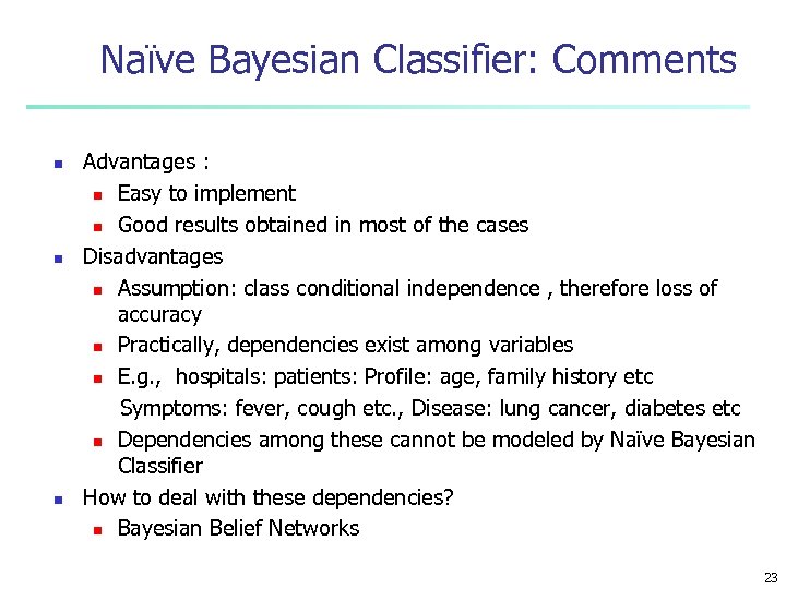Naïve Bayesian Classifier: Comments n n n Advantages : n Easy to implement n Good results obtained in most of the cases Disadvantages n Assumption: class conditional independence , therefore loss of accuracy n Practically, dependencies exist among variables n E. g. , hospitals: patients: Profile: age, family history etc Symptoms: fever, cough etc. , Disease: lung cancer, diabetes etc n Dependencies among these cannot be modeled by Naïve Bayesian Classifier How to deal with these dependencies? n Bayesian Belief Networks 23

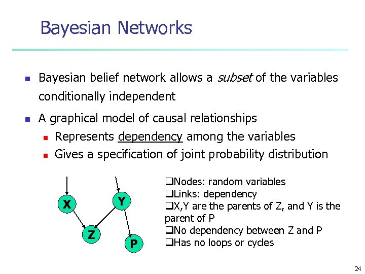Bayesian Networks n Bayesian belief network allows a subset of the variables conditionally independent n A graphical model of causal relationships n n Represents dependency among the variables Gives a specification of joint probability distribution Y X Z P q. Nodes: random variables q. Links: dependency q. X, Y are the parents of Z, and Y is the parent of P q. No dependency between Z and P q. Has no loops or cycles 24

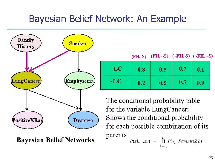Bayesian Belief Network: An Example Family History Smoker (FH, S) (FH, ~S) (~FH, ~S) LC Lung. Cancer Positive. XRay Emphysema Dyspnea Bayesian Belief Networks 0. 8 0. 5 0. 7 0. 1 ~LC 0. 2 0. 5 0. 3 0. 9 The conditional probability table for the variable Lung. Cancer: Shows the conditional probability for each possible combination of its parents 25

Learning Bayesian Networks n n Several cases n Given both the network structure and all variables observable: learn only the CPTs n Network structure known, some hidden variables: method of gradient descent, analogous to neural network learning n Network structure unknown, all variables observable: search through the model space to reconstruct graph topology n Unknown structure, all hidden variables: no good algorithms known for this purpose D. Heckerman, Bayesian networks for data mining 26

Chapter 7. Classification and Prediction n n What is classification? What is prediction? Issues regarding classification and prediction Classification by decision tree induction Bayesian Classification by Neural Networks Classification by Support Vector Machines (SVM) Classification based on concepts from association rule mining Other Classification Methods Prediction Classification accuracy Summary 27

Other Classification Methods n k-nearest neighbor classifier n case-based reasoning n Genetic algorithm n Rough set approach n Fuzzy set approaches 28

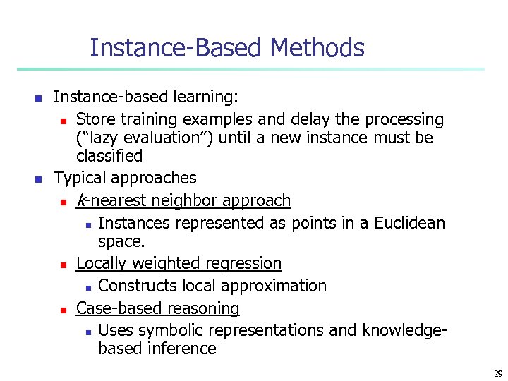Instance-Based Methods n n Instance-based learning: n Store training examples and delay the processing (“lazy evaluation”) until a new instance must be classified Typical approaches n k-nearest neighbor approach n Instances represented as points in a Euclidean space. n Locally weighted regression n Constructs local approximation n Case-based reasoning n Uses symbolic representations and knowledgebased inference 29

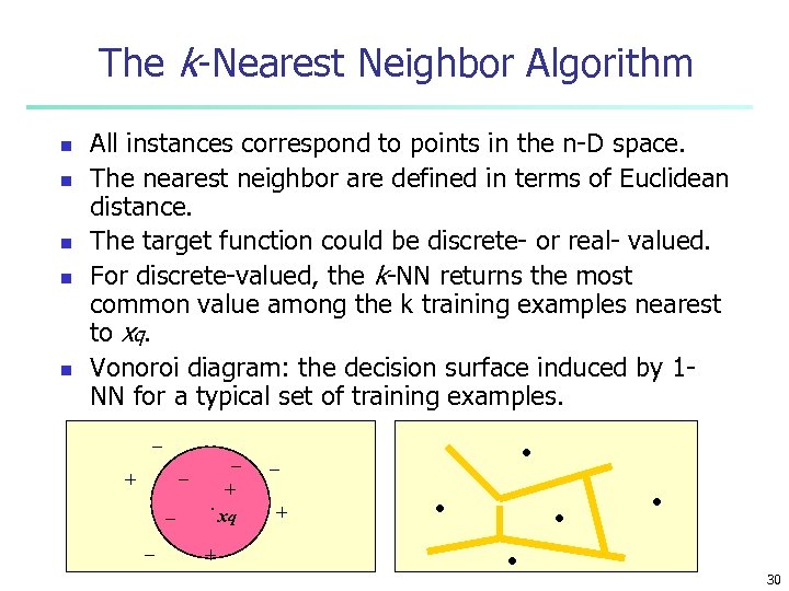The k-Nearest Neighbor Algorithm n n n All instances correspond to points in the n-D space. The nearest neighbor are defined in terms of Euclidean distance. The target function could be discrete- or real- valued. For discrete-valued, the k-NN returns the most common value among the k training examples nearest to xq. Vonoroi diagram: the decision surface induced by 1 NN for a typical set of training examples. _ _ _ + _ _ . + + xq . _ + . . 30

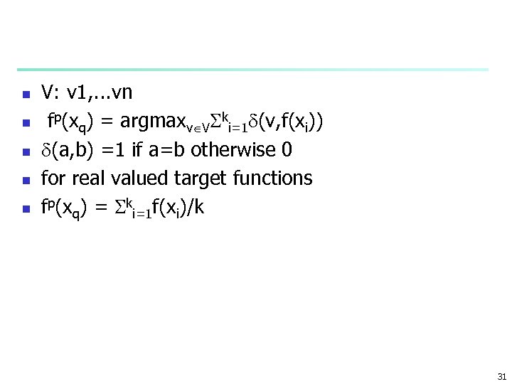n n n V: v 1, . . . vn fp(xq) = argmaxv V ki=1 (v, f(xi)) (a, b) =1 if a=b otherwise 0 for real valued target functions fp(xq) = ki=1 f(xi)/k 31

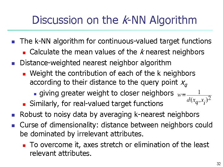Discussion on the k-NN Algorithm n n The k-NN algorithm for continuous-valued target functions n Calculate the mean values of the k nearest neighbors Distance-weighted nearest neighbor algorithm n Weight the contribution of each of the k neighbors according to their distance to the query point xq n giving greater weight to closer neighbors n Similarly, for real-valued target functions Robust to noisy data by averaging k-nearest neighbors Curse of dimensionality: distance between neighbors could be dominated by irrelevant attributes. n To overcome it, axes stretch or elimination of the least relevant attributes. 32

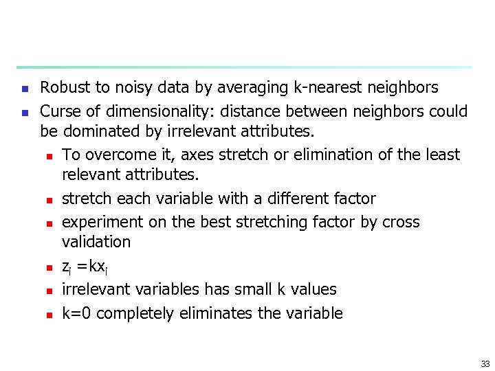n n Robust to noisy data by averaging k-nearest neighbors Curse of dimensionality: distance between neighbors could be dominated by irrelevant attributes. n To overcome it, axes stretch or elimination of the least relevant attributes. n stretch each variable with a different factor n experiment on the best stretching factor by cross validation n zi =kxi n irrelevant variables has small k values n k=0 completely eliminates the variable 33

Chapter 7. Classification and Prediction n n What is classification? What is prediction? Issues regarding classification and prediction Classification by decision tree induction Bayesian Classification by Neural Networks Classification by Support Vector Machines (SVM) Classification based on concepts from association rule mining Other Classification Methods Prediction Classification accuracy Summary 34

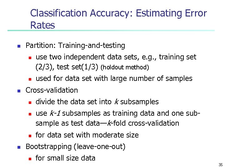Classification Accuracy: Estimating Error Rates n Partition: Training-and-testing n n n used for data set with large number of samples Cross-validation n n use two independent data sets, e. g. , training set (2/3), test set(1/3) (holdout method) divide the data set into k subsamples use k-1 subsamples as training data and one subsample as test data—k-fold cross-validation for data set with moderate size Bootstrapping (leave-one-out) n for small size data 35

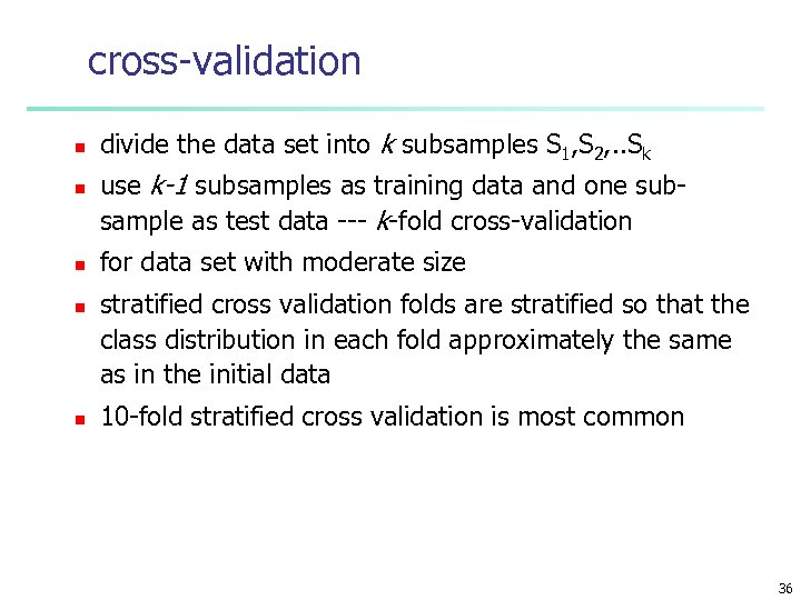cross-validation n n divide the data set into k subsamples S 1, S 2, . . Sk use k-1 subsamples as training data and one subsample as test data --- k-fold cross-validation for data set with moderate size stratified cross validation folds are stratified so that the class distribution in each fold approximately the same as in the initial data 10 -fold stratified cross validation is most common 36

leave-one-out n n for small size data k = S sample size in cross validation n one sample is used for testing n S-1 for training n repeat for each sample 37

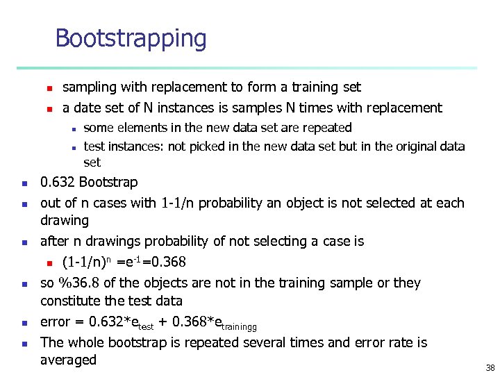Bootstrapping n n sampling with replacement to form a training set a date set of N instances is samples N times with replacement n n n n some elements in the new data set are repeated test instances: not picked in the new data set but in the original data set 0. 632 Bootstrap out of n cases with 1 -1/n probability an object is not selected at each drawing after n drawings probability of not selecting a case is n -1 n (1 -1/n) =e =0. 368 so %36. 8 of the objects are not in the training sample or they constitute the test data error = 0. 632*etest + 0. 368*etrainingg The whole bootstrap is repeated several times and error rate is averaged 38

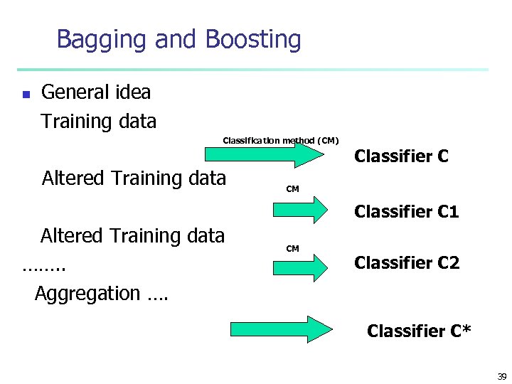Bagging and Boosting n General idea Training data Classification method (CM) Altered Training data Classifier C CM Classifier C 1 Altered Training data ……. . Aggregation …. CM Classifier C 2 Classifier C* 39

Bagging n n n Given a set S of s samples Generate a bootstrap sample T from S. Cases in S may not appear in T or may appear more than once. Repeat this sampling procedure, getting a sequence of k independent training sets A corresponding sequence of classifiers C 1, C 2, …, Ck is constructed for each of these training sets, by using the same classification algorithm To classify an unknown sample X, let each classifier predict or vote The Bagged Classifier C* counts the votes and assigns X to the class with the “most” votes 40

Increasing classifier accuracy-Bagging WF pp 250 -253 n n n n Bagging take t samples from data S sampling with replacement n each case may occur more than ones a new classifier Ct is learned for each set St Form the bagged classifier C* by voting classifiers equally n the majority rule For continuous valued prediction problems n take the average of each predictor 41

Increasing classifier accuracy. Boosting WF pp 254 -258 n n n Boosting increases classification accuracy n Applicable to decision trees or Bayesian classifier Learn a series of classifiers, where each classifier in the series pays more attention to the examples misclassified by its predecessor Boosting requires only linear time and constant space 42

Boosting Technique — Algorithm n Assign every example an equal weight 1/N n For t = 1, 2, …, T Do Obtain a hypothesis (classifier) h(t) under w(t) n Calculate the error of h(t) and re-weight the examples based on the error. Each classifier is dependent on the previous ones. Samples that are incorrectly predicted are weighted more heavily (t+1) to sum to 1 (weights assigned to n Normalize w different classifiers sum to 1) Output a weighted sum of all the hypothesis, with each hypothesis weighted according to its accuracy on the training set n n 43

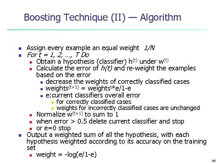Boosting Technique (II) — Algorithm n n Assign every example an equal weight 1/N For t = 1, 2, …, T Do n n Obtain a hypothesis (classifier) h(t) under w(t) Calculate the error of h(t) and re-weight the examples based on the error n decrease the weights of correctly classified cases (t+1) = weightst*e/1 -e n weights n e: current classifiers overall error n n for correctly classified cases weights for incorrectly classified cases are unchanged Normalize w(t+1) to sum to 1 n when error > 0. 5 delete current classifier and stop n or e=0 stop Output a weighted sum of all the hypothesis, with each hypothesis weighted according to its accuracy on the training set n weight = -log(e/1 -e) n n 44

Bagging and Boosting n n n Experiments with a new boosting algorithm, freund et al (Ada. Boost ) Bagging Predictors, Brieman Boosting Naïve Bayesian Learning on large subset of MEDLINE, W. Wilbur 45

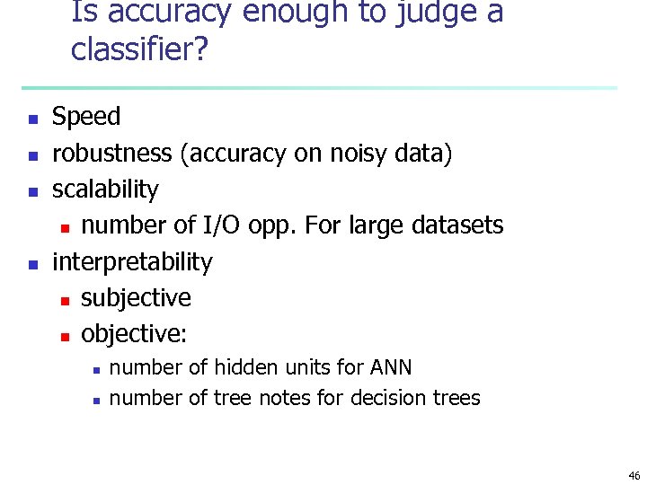Is accuracy enough to judge a classifier? n n Speed robustness (accuracy on noisy data) scalability n number of I/O opp. For large datasets interpretability n subjective n objective: n n number of hidden units for ANN number of tree notes for decision trees 46

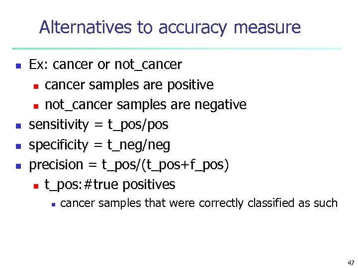Alternatives to accuracy measure n n Ex: cancer or not_cancer n cancer samples are positive n not_cancer samples are negative sensitivity = t_pos/pos specificity = t_neg/neg precision = t_pos/(t_pos+f_pos) n t_pos: #true positives n cancer samples that were correctly classified as such 47

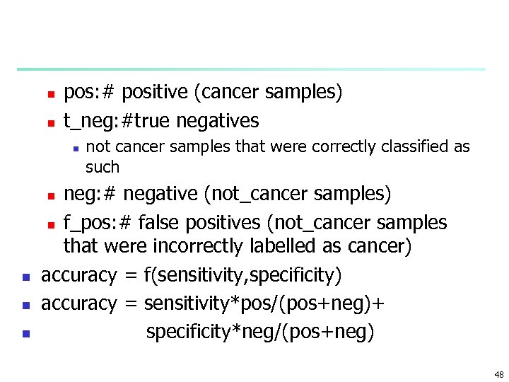n n pos: # positive (cancer samples) t_neg: #true negatives n not cancer samples that were correctly classified as such neg: # negative (not_cancer samples) n f_pos: # false positives (not_cancer samples that were incorrectly labelled as cancer) accuracy = f(sensitivity, specificity) accuracy = sensitivity*pos/(pos+neg)+ specificity*neg/(pos+neg) n n 48

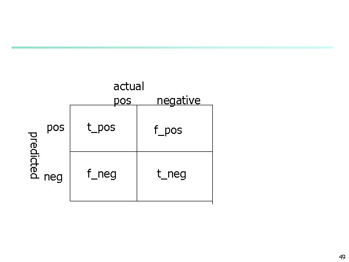actual pos negative predicted pos t_pos f_pos neg f_neg t_neg 49

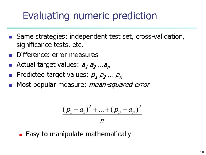Evaluating numeric prediction n n Same strategies: independent test set, cross-validation, significance tests, etc. Difference: error measures Actual target values: a 1 a 2 …an Predicted target values: p 1 p 2 … pn Most popular measure: mean-squared error n Easy to manipulate mathematically 50

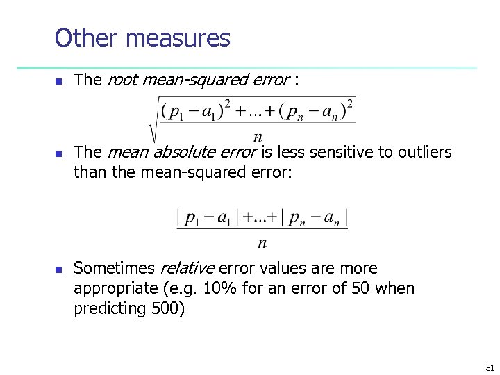Other measures n n n The root mean-squared error : The mean absolute error is less sensitive to outliers than the mean-squared error: Sometimes relative error values are more appropriate (e. g. 10% for an error of 50 when predicting 500) 51

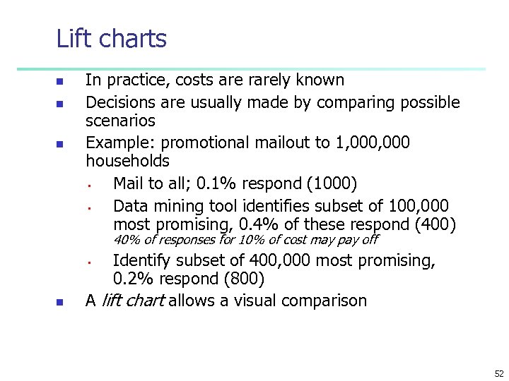Lift charts n n n In practice, costs are rarely known Decisions are usually made by comparing possible scenarios Example: promotional mailout to 1, 000 households • Mail to all; 0. 1% respond (1000) • Data mining tool identifies subset of 100, 000 most promising, 0. 4% of these respond (400) 40% of responses for 10% of cost may pay off Identify subset of 400, 000 most promising, 0. 2% respond (800) A lift chart allows a visual comparison • n 52

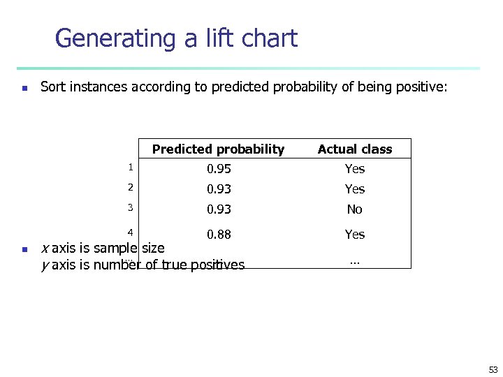Generating a lift chart n Sort instances according to predicted probability of being positive: Predicted probability 1 0. 95 Yes 2 0. 93 Yes 3 0. 93 No 4 n Actual class 0. 88 Yes x axis is sample size … … y axis is number of true positives … 53

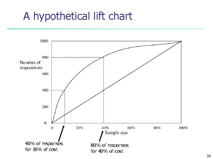A hypothetical lift chart 40% of responses for 10% of cost 80% of responses for 40% of cost 54

Chapter 7. Classification and Prediction n n What is classification? What is prediction? Issues regarding classification and prediction Classification by decision tree induction Bayesian Classification by Neural Networks Classification by Support Vector Machines (SVM) Classification based on concepts from association rule mining Other Classification Methods Prediction Classification accuracy Summary 55

Summary n Classification is an extensively studied problem (mainly in statistics, machine learning & neural networks) n Classification is probably one of the most widely used data mining techniques with a lot of extensions n Scalability is still an important issue for database applications: thus combining classification with database techniques should be a promising topic n Research directions: classification of non-relational data, e. g. , text, spatial, multimedia, etc. . 56

References (1) n n n n C. Apte and S. Weiss. Data mining with decision trees and decision rules. Future Generation Computer Systems, 13, 1997. L. Breiman, J. Friedman, R. Olshen, and C. Stone. Classification and Regression Trees. Wadsworth International Group, 1984. C. J. C. Burges. A Tutorial on Support Vector Machines for Pattern Recognition. Data Mining and Knowledge Discovery, 2(2): 121 -168, 1998. P. K. Chan and S. J. Stolfo. Learning arbiter and combiner trees from partitioned data for scaling machine learning. In Proc. 1 st Int. Conf. Knowledge Discovery and Data Mining (KDD'95), pages 39 -44, Montreal, Canada, August 1995. U. M. Fayyad. Branching on attribute values in decision tree generation. In Proc. 1994 AAAI Conf. , pages 601 -606, AAAI Press, 1994. J. Gehrke, R. Ramakrishnan, and V. Ganti. Rainforest: A framework for fast decision tree construction of large datasets. In Proc. 1998 Int. Conf. Very Large Data Bases, pages 416 -427, New York, NY, August 1998. J. Gehrke, V. Gant, R. Ramakrishnan, and W. -Y. Loh, BOAT -- Optimistic Decision Tree Construction. In SIGMOD'99 , Philadelphia, Pennsylvania, 1999 57

References (2) n M. Kamber, L. Winstone, W. Gong, S. Cheng, and J. Han. Generalization and decision tree induction: Efficient classification in data mining. In Proc. 1997 Int. Workshop Research Issues on Data Engineering (RIDE'97), Birmingham, England, April 1997. n B. Liu, W. Hsu, and Y. Ma. Integrating Classification and Association Rule Mining. Proc. 1998 Int. Conf. Knowledge Discovery and Data Mining (KDD'98) New York, NY, Aug. 1998. n W. Li, J. Han, and J. Pei, CMAR: Accurate and Efficient Classification Based on Multiple Class-Association Rules, , Proc. 2001 Int. Conf. on Data Mining (ICDM'01), San Jose, CA, Nov. 2001. n J. Magidson. The Chaid approach to segmentation modeling: Chi-squared automatic interaction detection. In R. P. Bagozzi, editor, Advanced Methods of Marketing Research, pages 118 -159. Blackwell Business, Cambridge Massechusetts, 1994. n M. Mehta, R. Agrawal, and J. Rissanen. SLIQ : A fast scalable classifier for data mining. (EDBT'96), Avignon, France, March 1996. 58

References (3) n n n n T. M. Mitchell. Machine Learning. Mc. Graw Hill, 1997. S. K. Murthy, Automatic Construction of Decision Trees from Data: A Multi-Diciplinary Survey, Data Mining and Knowledge Discovery 2(4): 345 -389, 1998 J. R. Quinlan. Induction of decision trees. Machine Learning, 1: 81 -106, 1986. J. R. Quinlan. Bagging, boosting, and c 4. 5. In Proc. 13 th Natl. Conf. on Artificial Intelligence (AAAI'96), 725 -730, Portland, OR, Aug. 1996. R. Rastogi and K. Shim. Public: A decision tree classifer that integrates building and pruning. In Proc. 1998 Int. Conf. Very Large Data Bases, 404 -415, New York, NY, August 1998. J. Shafer, R. Agrawal, and M. Mehta. SPRINT : A scalable parallel classifier for data mining. In Proc. 1996 Int. Conf. Very Large Data Bases, 544 -555, Bombay, India, Sept. 1996. S. M. Weiss and C. A. Kulikowski. Computer Systems that Learn: Classification and Prediction Methods from Statistics, Neural Nets, Machine Learning, and Expert Systems. Morgan Kaufman, 1991. S. M. Weiss and N. Indurkhya. Predictive Data Mining. Morgan Kaufmann, 1997. 59

www. cs. uiuc. edu/~hanj Thank you !!! 60