Data Mining Concepts and Techniques Chapter 2

Data Mining: Concepts and Techniques — Chapter 2 — Dr. Maher Abuhamdeh Statistical 16 March 2018 Data Mining: Concepts and Techniques 1

Mining Data Descriptive Characteristics n Motivation n n Data dispersion characteristics n n To better understand the data: central tendency, variation and spread median, max, min, quantiles, outliers, variance, etc. Numerical dimensions correspond to sorted intervals n n n Data dispersion: analyzed with multiple granularities of precision Boxplot or quantile analysis on sorted intervals Dispersion analysis on computed measures n Folding measures into numerical dimensions n Boxplot or quantile analysis on the transformed cube 16 March 2018 Data Mining: Concepts and Techniques 2

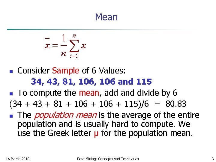Mean Consider Sample of 6 Values: 34, 43, 81, 106 and 115 n To compute the mean, add and divide by 6 (34 + 43 + 81 + 106 + 115)/6 = 80. 83 n The population mean is the average of the entire population and is usually hard to compute. We use the Greek letter μ for the population mean. n 16 March 2018 Data Mining: Concepts and Techniques 3

Mode n n The mode of a set of data is the number with the highest frequency. In the above example 106 is the mode, since it occurs twice and the rest of the outcomes occur only once. 16 March 2018 Data Mining: Concepts and Techniques 4

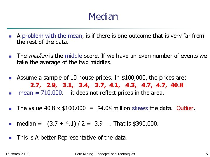Median n n A problem with the mean, is if there is one outcome that is very far from the rest of the data. The median is the middle score. If we have an even number of events we take the average of the two middles. n Assume a sample of 10 house prices. In $100, 000, the prices are: 2. 7, 2. 9, 3. 1, 3. 4, 3. 7, 4. 1, 4. 3, 4. 7, 40. 8 mean = 710, 000. it does not reflect prices in the area. n The value 40. 8 x $100, 000 = $4. 08 million skews the data. Outlier. n n n median = (3. 7 + 4. 1) / 2 = 3. 9 . . That is $390, 000. This is A better Representative of the data. 16 March 2018 Data Mining: Concepts and Techniques 5

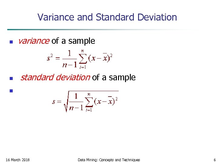Variance and Standard Deviation n variance of a sample n standard deviation of a sample n 16 March 2018 Data Mining: Concepts and Techniques 6

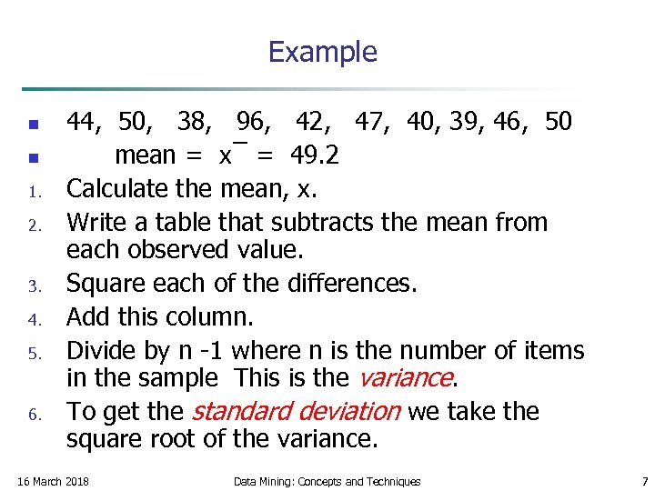Example n n 1. 2. 3. 4. 5. 6. 44, 50, 38, 96, 42, 47, 40, 39, 46, 50 mean = x = 49. 2 Calculate the mean, x. Write a table that subtracts the mean from each observed value. Square each of the differences. Add this column. Divide by n -1 where n is the number of items in the sample This is the variance. To get the standard deviation we take the square root of the variance. 16 March 2018 Data Mining: Concepts and Techniques 7

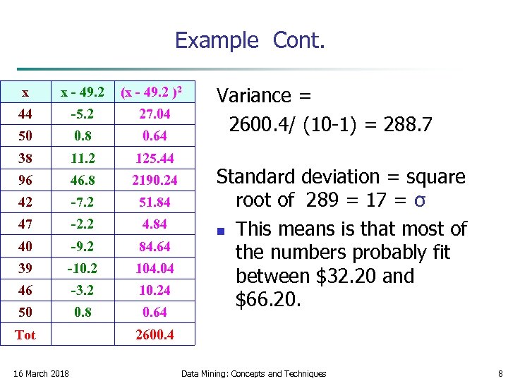Example Cont. x x - 49. 2 (x - 49. 2 )2 44 -5. 2 27. 04 50 0. 8 0. 64 38 11. 2 125. 44 96 46. 8 2190. 24 42 -7. 2 51. 84 47 -2. 2 4. 84 40 -9. 2 84. 64 39 -10. 2 104. 04 46 -3. 2 10. 24 50 0. 8 0. 64 Tot Variance = 2600. 4/ (10 -1) = 288. 7 Standard deviation = square root of 289 = 17 = σ n This means is that most of the numbers probably fit between $32. 20 and $66. 20. 2600. 4 16 March 2018 Data Mining: Concepts and Techniques 8

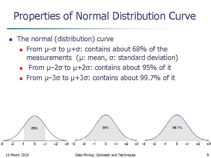Properties of Normal Distribution Curve n The normal (distribution) curve n From μ–σ to μ+σ: contains about 68% of the measurements (μ: mean, σ: standard deviation) n From μ– 2σ to μ+2σ: contains about 95% of it n From μ– 3σ to μ+3σ: contains about 99. 7% of it 16 March 2018 Data Mining: Concepts and Techniques 9

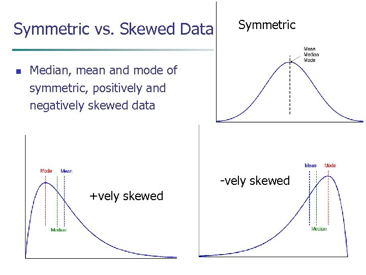Symmetric vs. Skewed Data n Median, mean and mode of symmetric, positively and negatively skewed data -vely skewed +vely skewed 16 March 2018 Data Mining: Concepts and Techniques 10

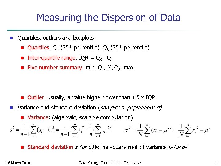Measuring the Dispersion of Data n Quartiles, outliers and boxplots n n Inter-quartile range: IQR = Q 3 – Q 1 n Five number summary: min, Q 1, M, Q 3, max n n Quartiles: Q 1 (25 th percentile), Q 3 (75 th percentile) Outlier: usually, a value higher/lower than 1. 5 x IQR Variance and standard deviation (sample: s, population: σ) n Variance: (algebraic, scalable computation) n Standard deviation s (or σ) is the square root of variance s 2 (or σ2) 16 March 2018 Data Mining: Concepts and Techniques 11

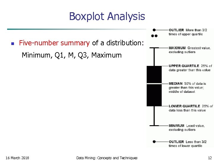Boxplot Analysis n Five-number summary of a distribution: Minimum, Q 1, M, Q 3, Maximum 16 March 2018 Data Mining: Concepts and Techniques 12

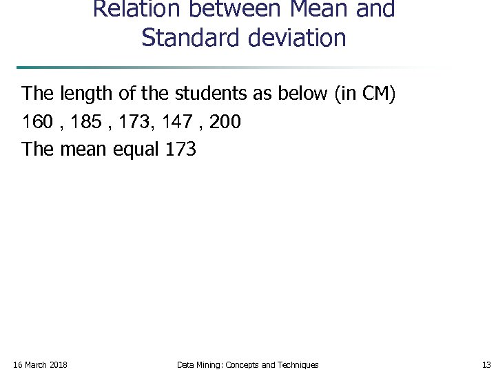Relation between Mean and Standard deviation The length of the students as below (in CM) 160 , 185 , 173, 147 , 200 The mean equal 173 16 March 2018 Data Mining: Concepts and Techniques 13

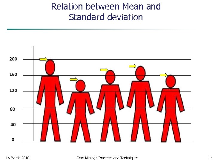Relation between Mean and Standard deviation 16 March 2018 Data Mining: Concepts and Techniques 14

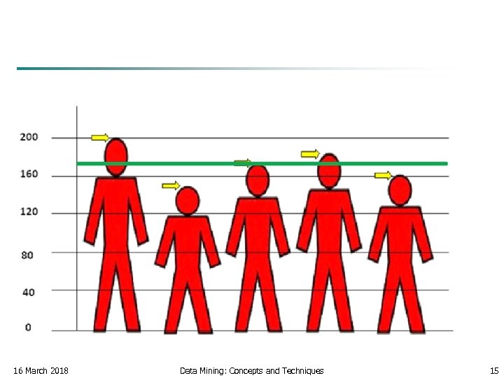16 March 2018 Data Mining: Concepts and Techniques 15

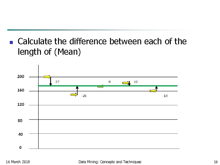n Calculate the difference between each of the length of (Mean) 16 March 2018 Data Mining: Concepts and Techniques 16

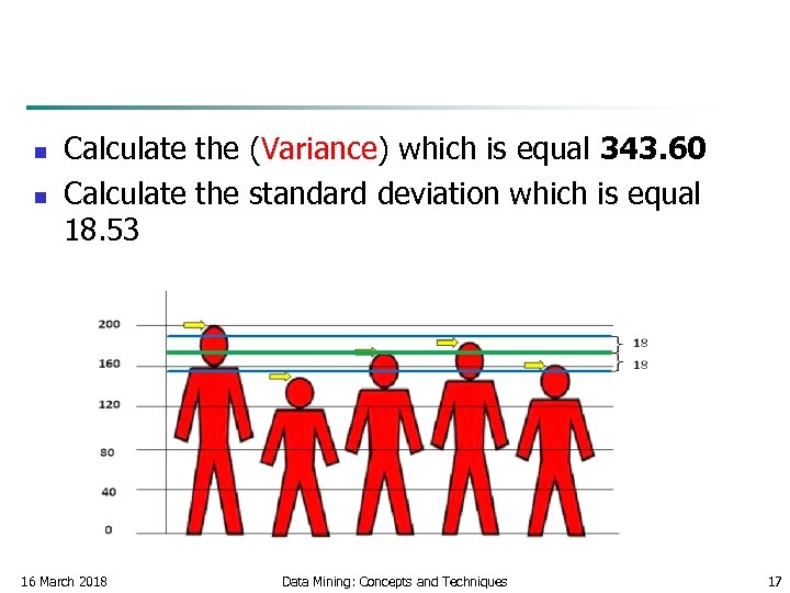n n Calculate the (Variance) which is equal 343. 60 Calculate the standard deviation which is equal 18. 53 16 March 2018 Data Mining: Concepts and Techniques 17

n n n The first student is unusually long The second student is short The others are considered as normal lengths If Mean close with Standard deviation increased accuracy (homogeneity) If Mean far away with Standard deviation decreased accuracy (non-homogeneity) 16 March 2018 Data Mining: Concepts and Techniques 18

How to Handle Noisy Data? 1. Binning n first sort data and partition into (equal-frequency) bins n then one can smooth by bin means, smooth by bin median, smooth by bin boundaries, etc. 16 March 2018 Data Mining: Concepts and Techniques 19

Simple Discretization Methods: Binning n Equal-width (distance) partitioning n Divides the range into N intervals of equal size: uniform grid n if A and B are the lowest and highest values of the attribute, the width of intervals will be: W = (B –A)/N. n n n The most straightforward, but outliers may dominate presentation Skewed data is not handled well Equal-depth (frequency) partitioning n Divides the range into N intervals, each containing approximately same number of samples n Good data scaling n Managing categorical attributes can be tricky 16 March 2018 Data Mining: Concepts and Techniques 20

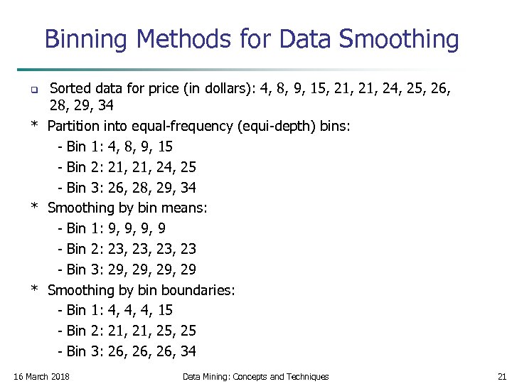Binning Methods for Data Smoothing Sorted data for price (in dollars): 4, 8, 9, 15, 21, 24, 25, 26, 28, 29, 34 * Partition into equal-frequency (equi-depth) bins: - Bin 1: 4, 8, 9, 15 - Bin 2: 21, 24, 25 - Bin 3: 26, 28, 29, 34 * Smoothing by bin means: - Bin 1: 9, 9, 9, 9 - Bin 2: 23, 23, 23 - Bin 3: 29, 29, 29 * Smoothing by bin boundaries: - Bin 1: 4, 4, 4, 15 - Bin 2: 21, 25, 25 - Bin 3: 26, 26, 34 q 16 March 2018 Data Mining: Concepts and Techniques 21

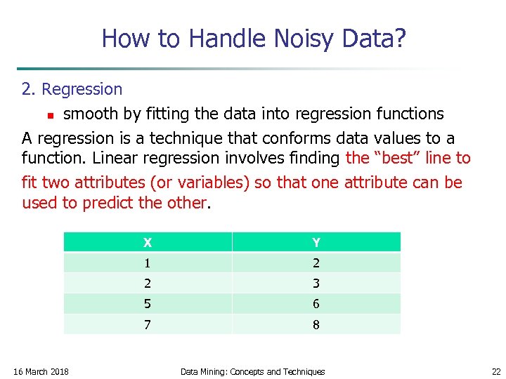How to Handle Noisy Data? 2. Regression n smooth by fitting the data into regression functions A regression is a technique that conforms data values to a function. Linear regression involves finding the “best” line to fit two attributes (or variables) so that one attribute can be used to predict the other. X 1 2 2 3 5 6 7 16 March 2018 Y 8 Data Mining: Concepts and Techniques 22

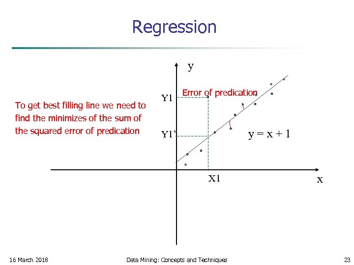Regression y Error of predication Y 1 To get best filling line we need to find the minimizes of the sum of the squared error of predication y=x+1 Y 1’ X 1 16 March 2018 Data Mining: Concepts and Techniques x 23

How to Handle Noisy Data? 3. Clustering Outliers may be detected by clustering, for example, where similar values are organized into groups, or “clusters. ” Intuitively, values that fall outside of the set of clusters may be considered outliers, then we need to remove them 16 March 2018 Data Mining: Concepts and Techniques 24

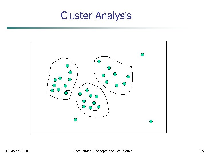Cluster Analysis 16 March 2018 Data Mining: Concepts and Techniques 25

Normalization n Normalization: scaled to fall within a small, specified range n n z-score normalization n n min-max normalization by decimal scaling Attribute/feature construction n 16 March 2018 New attributes constructed from the given ones Data Mining: Concepts and Techniques 26

Data Transformation: Normalization n n 1. 2. 3. Normalization : where the attribute data are scaled so as to fall within a small specified range such as [-1. 0 to 1. 0] or [0. 0 to 1. 0] We study three methods for normalization Min – max normalization z - score normalization Decimal scaling 16 March 2018 Data Mining: Concepts and Techniques 27

Data Transformation: Normalization n Min-max normalization: to [new_min. A, new_max. A] n n Z-score normalization (μ: mean, σ: standard deviation): n n Ex. Let income range $12, 000 to $98, 000 normalized to [0. 0, 1. 0]. Then $73, 600 is mapped to Ex. Let μ = 54, 000, σ = 16, 000. Then Normalization by decimal scaling Where j is the smallest integer such that Max(|ν’|) < 1 16 March 2018 Data Mining: Concepts and Techniques 28

Normalization by decimal scaling Example: Suppose values of A range from -986 to 917. The maximum absolute value of A is 986. To normalize by decimal scaling we divide each value by 1000 (j = 3) so that -986 normalizes to -0. 986 n 16 March 2018 Data Mining: Concepts and Techniques 29

Remakes for three Normalization method n n Min-max normalization problem Out of bound error if a future input case for normalization falls outside of the original data range. Z-score normalization is useful when the actual min. and max. of attribute A are unknown or when there outliers that dominate the min – max normalization. 16 March 2018 Data Mining: Concepts and Techniques 30