Data Mining and Knowledge Acquizition Chapter 5

Data Mining and Knowledge Acquizition — Chapter 5 III — BIS 541 2016/2017 Summer 1

Chapter 7. Classification and Prediction n n Bayesian Classification Model Based Reasoning Collaborative Filtering Classification accuracy 2

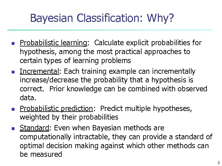Bayesian Classification: Why? n n Probabilistic learning: Calculate explicit probabilities for hypothesis, among the most practical approaches to certain types of learning problems Incremental: Each training example can incrementally increase/decrease the probability that a hypothesis is correct. Prior knowledge can be combined with observed data. Probabilistic prediction: Predict multiple hypotheses, weighted by their probabilities Standard: Even when Bayesian methods are computationally intractable, they can provide a standard of optimal decision making against which other methods can be measured 3

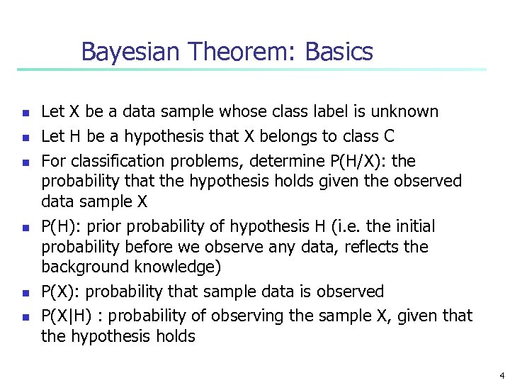Bayesian Theorem: Basics n n n Let X be a data sample whose class label is unknown Let H be a hypothesis that X belongs to class C For classification problems, determine P(H/X): the probability that the hypothesis holds given the observed data sample X P(H): prior probability of hypothesis H (i. e. the initial probability before we observe any data, reflects the background knowledge) P(X): probability that sample data is observed P(X|H) : probability of observing the sample X, given that the hypothesis holds 4

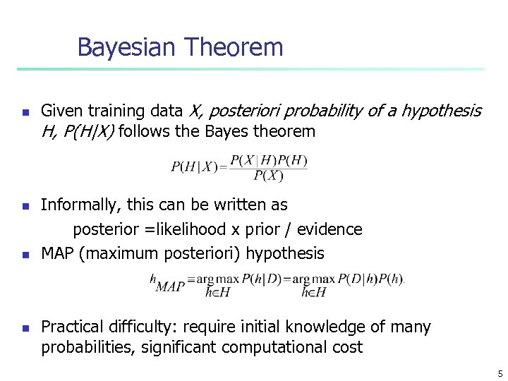Bayesian Theorem n n Given training data X, posteriori probability of a hypothesis H, P(H|X) follows the Bayes theorem Informally, this can be written as posterior =likelihood x prior / evidence MAP (maximum posteriori) hypothesis Practical difficulty: require initial knowledge of many probabilities, significant computational cost 5

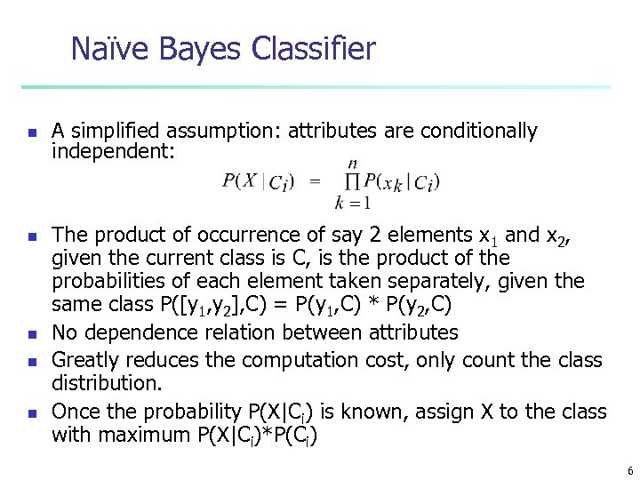Naïve Bayes Classifier n n n A simplified assumption: attributes are conditionally independent: The product of occurrence of say 2 elements x 1 and x 2, given the current class is C, is the product of the probabilities of each element taken separately, given the same class P([y 1, y 2], C) = P(y 1, C) * P(y 2, C) No dependence relation between attributes Greatly reduces the computation cost, only count the class distribution. Once the probability P(X|Ci) is known, assign X to the class with maximum P(X|Ci)*P(Ci) 6

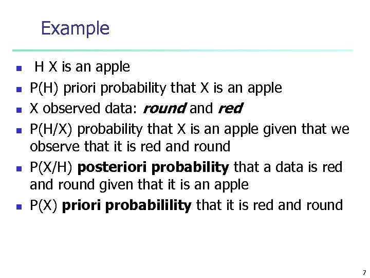Example n n n H X is an apple P(H) priori probability that X is an apple X observed data: round and red P(H/X) probability that X is an apple given that we observe that it is red and round P(X/H) posteriori probability that a data is red and round given that it is an apple P(X) priori probabilility that it is red and round 7

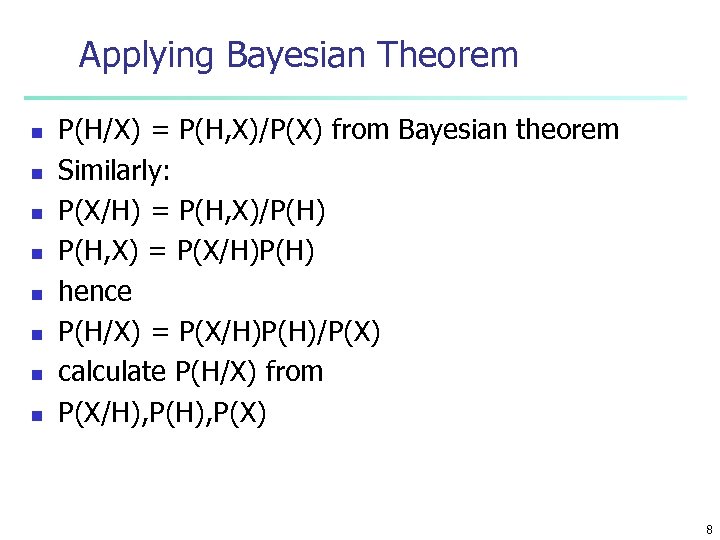Applying Bayesian Theorem n n n n P(H/X) = P(H, X)/P(X) from Bayesian theorem Similarly: P(X/H) = P(H, X)/P(H) P(H, X) = P(X/H)P(H) hence P(H/X) = P(X/H)P(H)/P(X) calculate P(H/X) from P(X/H), P(X) 8

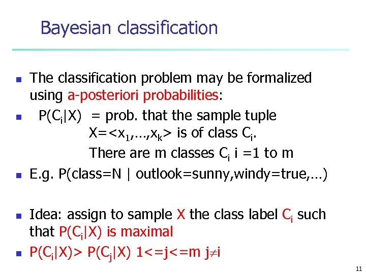Bayesian classification n n The classification problem may be formalized using a-posteriori probabilities: P(Ci|X) = prob. that the sample tuple X= is of class Ci. There are m classes Ci i =1 to m E. g. P(class=N | outlook=sunny, windy=true, …) Idea: assign to sample X the class label Ci such that P(Ci|X) is maximal P(Ci|X)> P(Cj|X) 1<=j<=m j i 11

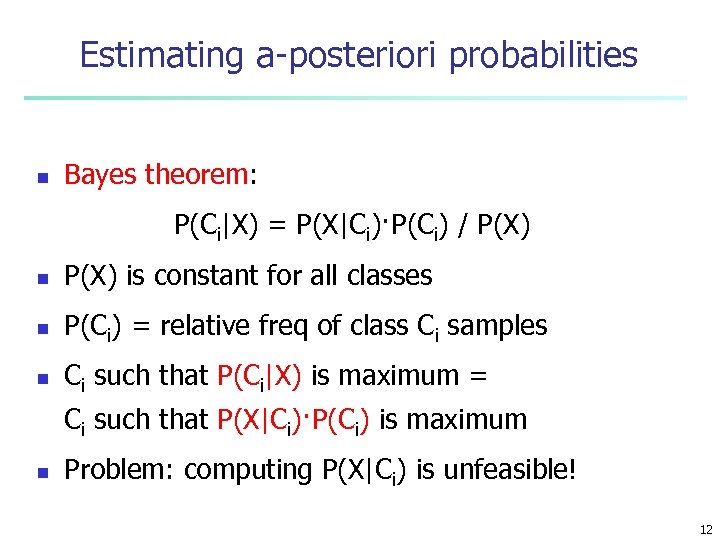Estimating a-posteriori probabilities n Bayes theorem: P(Ci|X) = P(X|Ci)·P(Ci) / P(X) n P(X) is constant for all classes n P(Ci) = relative freq of class Ci samples n Ci such that P(Ci|X) is maximum = Ci such that P(X|Ci)·P(Ci) is maximum n Problem: computing P(X|Ci) is unfeasible! 12

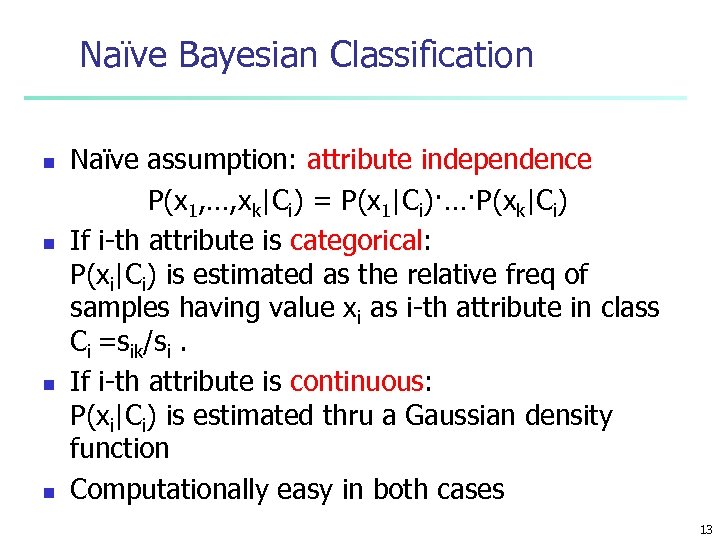Naïve Bayesian Classification n n Naïve assumption: attribute independence P(x 1, …, xk|Ci) = P(x 1|Ci)·…·P(xk|Ci) If i-th attribute is categorical: P(xi|Ci) is estimated as the relative freq of samples having value xi as i-th attribute in class Ci =sik/si. If i-th attribute is continuous: P(xi|Ci) is estimated thru a Gaussian density function Computationally easy in both cases 13

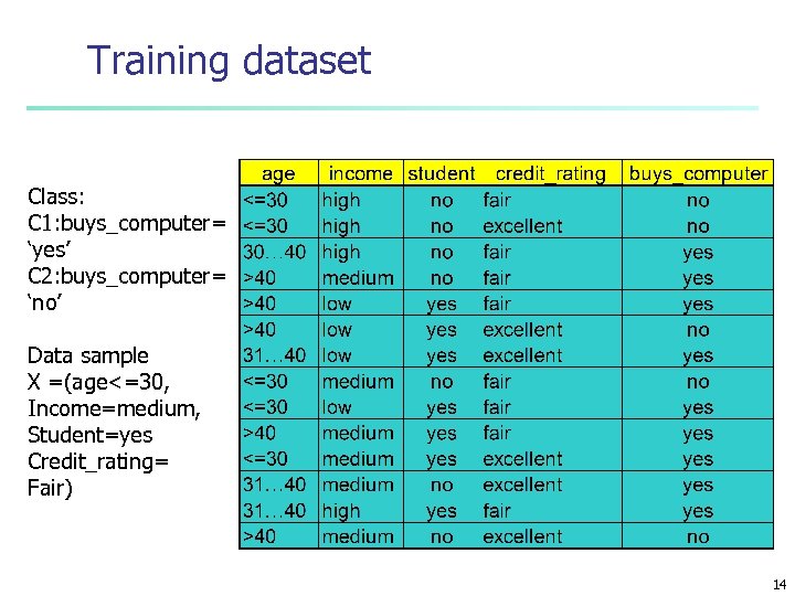Training dataset Class: C 1: buys_computer= ‘yes’ C 2: buys_computer= ‘no’ Data sample X =(age<=30, Income=medium, Student=yes Credit_rating= Fair) 14

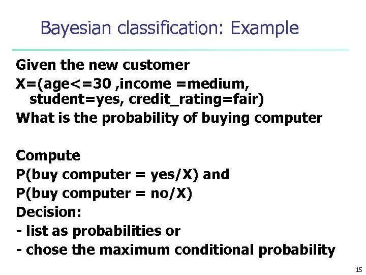Bayesian classification: Example Given the new customer X=(age<=30 , income =medium, student=yes, credit_rating=fair) What is the probability of buying computer Compute P(buy computer = yes/X) and P(buy computer = no/X) Decision: - list as probabilities or - chose the maximum conditional probability 15

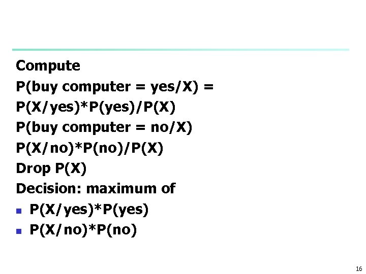Compute P(buy computer = yes/X) = P(X/yes)*P(yes)/P(X) P(buy computer = no/X) P(X/no)*P(no)/P(X) Drop P(X) Decision: maximum of n P(X/yes)*P(yes) n P(X/no)*P(no) 16

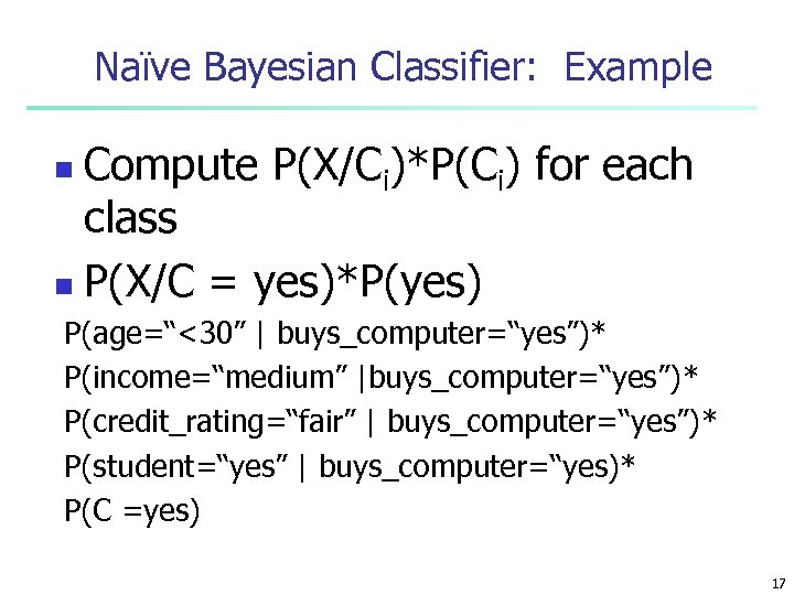Naïve Bayesian Classifier: Example Compute P(X/Ci)*P(Ci) for each class n P(X/C = yes)*P(yes) n P(age=“<30” | buys_computer=“yes”)* P(income=“medium” |buys_computer=“yes”)* P(credit_rating=“fair” | buys_computer=“yes”)* P(student=“yes” | buys_computer=“yes)* P(C =yes) 17

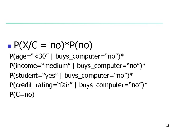n P(X/C = no)*P(no) P(age=“<30” | buys_computer=“no”)* P(income=“medium” | buys_computer=“no”)* P(student=“yes” | buys_computer=“no”)* P(credit_rating=“fair” | buys_computer=“no”)* P(C=no) 18

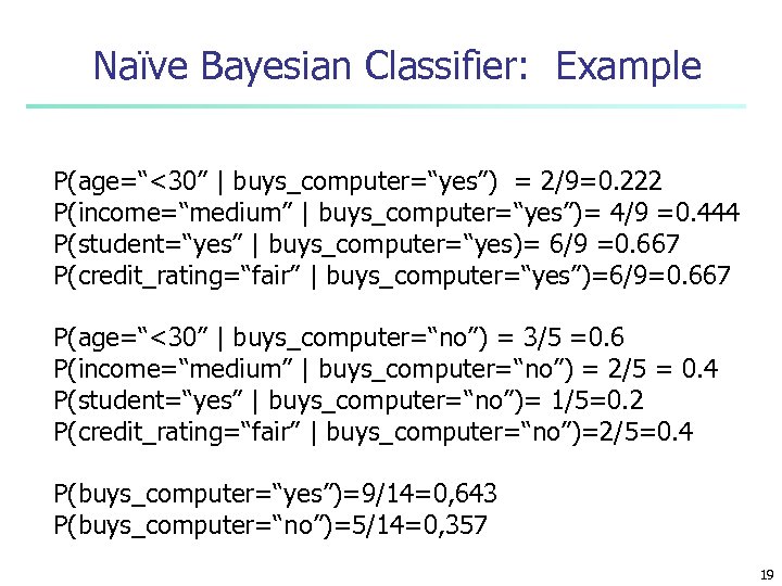Naïve Bayesian Classifier: Example P(age=“<30” | buys_computer=“yes”) = 2/9=0. 222 P(income=“medium” | buys_computer=“yes”)= 4/9 =0. 444 P(student=“yes” | buys_computer=“yes)= 6/9 =0. 667 P(credit_rating=“fair” | buys_computer=“yes”)=6/9=0. 667 P(age=“<30” | buys_computer=“no”) = 3/5 =0. 6 P(income=“medium” | buys_computer=“no”) = 2/5 = 0. 4 P(student=“yes” | buys_computer=“no”)= 1/5=0. 2 P(credit_rating=“fair” | buys_computer=“no”)=2/5=0. 4 P(buys_computer=“yes”)=9/14=0, 643 P(buys_computer=“no”)=5/14=0, 357 19

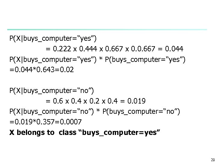P(X|buys_computer=“yes”) = 0. 222 x 0. 444 x 0. 667 x 0. 0. 667 = 0. 044 P(X|buys_computer=“yes”) * P(buys_computer=“yes”) =0. 044*0. 643=0. 02 P(X|buys_computer=“no”) = 0. 6 x 0. 4 x 0. 2 x 0. 4 = 0. 019 P(X|buys_computer=“no”) * P(buys_computer=“no”) =0. 019*0. 357=0. 0007 X belongs to class “buys_computer=yes” 20

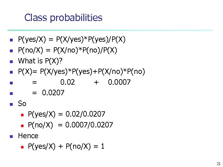Class probabilities n n n n P(yes/X) = P(X/yes)*P(yes)/P(X) P(no/X) = P(X/no)*P(no)/P(X) What is P(X)? P(X)= P(X/yes)*P(yes)+P(X/no)*P(no) = 0. 02 + 0. 0007 = 0. 0207 So n P(yes/X) = 0. 02/0. 0207 n P(no/X) = 0. 0007/0. 0207 Hence n P(yes/X) + P(no/X) = 1 21

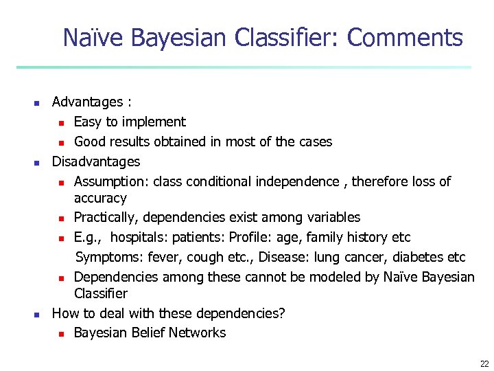Naïve Bayesian Classifier: Comments n n n Advantages : n Easy to implement n Good results obtained in most of the cases Disadvantages n Assumption: class conditional independence , therefore loss of accuracy n Practically, dependencies exist among variables n E. g. , hospitals: patients: Profile: age, family history etc Symptoms: fever, cough etc. , Disease: lung cancer, diabetes etc n Dependencies among these cannot be modeled by Naïve Bayesian Classifier How to deal with these dependencies? n Bayesian Belief Networks 22

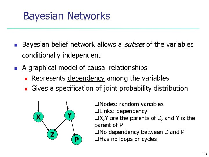Bayesian Networks n Bayesian belief network allows a subset of the variables conditionally independent n A graphical model of causal relationships n n Represents dependency among the variables Gives a specification of joint probability distribution Y X Z P q. Nodes: random variables q. Links: dependency q. X, Y are the parents of Z, and Y is the parent of P q. No dependency between Z and P q. Has no loops or cycles 23

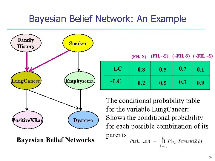Bayesian Belief Network: An Example Family History Smoker (FH, S) (FH, ~S) (~FH, ~S) LC Lung. Cancer Positive. XRay Emphysema Dyspnea Bayesian Belief Networks 0. 8 0. 5 0. 7 0. 1 ~LC 0. 2 0. 5 0. 3 0. 9 The conditional probability table for the variable Lung. Cancer: Shows the conditional probability for each possible combination of its parents 24

Learning Bayesian Networks n n Several cases n Given both the network structure and all variables observable: learn only the CPTs n Network structure known, some hidden variables: method of gradient descent, analogous to neural network learning n Network structure unknown, all variables observable: search through the model space to reconstruct graph topology n Unknown structure, all hidden variables: no good algorithms known for this purpose D. Heckerman, Bayesian networks for data mining 25

Chapter 7. Classification and Prediction n n Bayesian Classification Model Based Reasoning Collaborative Filtering Classification accuracy 26

Other Classification Methods n k-nearest neighbor classifier n case-based reasoning n Genetic algorithm n Rough set approach n Fuzzy set approaches 27

Instance-Based Methods n n Instance-based learning: n Store training examples and delay the processing (“lazy evaluation”) until a new instance must be classified Typical approaches n k-nearest neighbor approach n Instances represented as points in a Euclidean space. n Locally weighted regression n Constructs local approximation n Case-based reasoning n Uses symbolic representations and knowledgebased inference 28

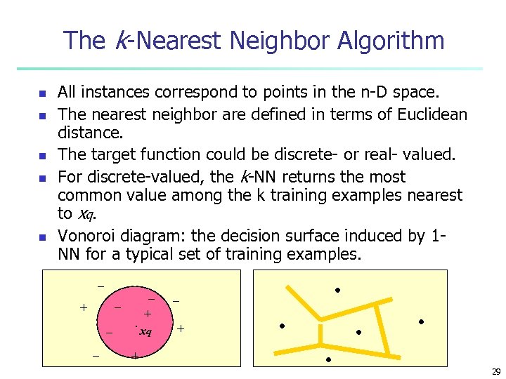The k-Nearest Neighbor Algorithm n n n All instances correspond to points in the n-D space. The nearest neighbor are defined in terms of Euclidean distance. The target function could be discrete- or real- valued. For discrete-valued, the k-NN returns the most common value among the k training examples nearest to xq. Vonoroi diagram: the decision surface induced by 1 NN for a typical set of training examples. _ _ _ + _ _ . + + xq . _ + . . 29

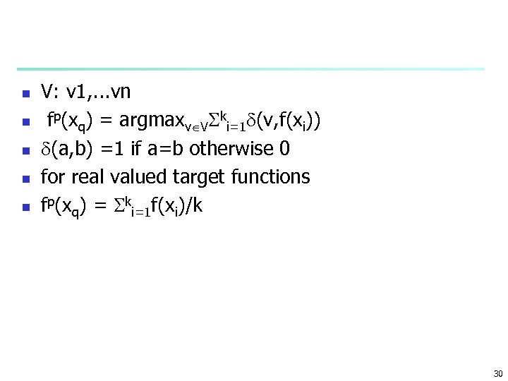n n n V: v 1, . . . vn fp(xq) = argmaxv V ki=1 (v, f(xi)) (a, b) =1 if a=b otherwise 0 for real valued target functions fp(xq) = ki=1 f(xi)/k 30

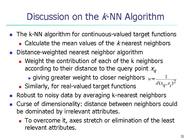Discussion on the k-NN Algorithm n n The k-NN algorithm for continuous-valued target functions n Calculate the mean values of the k nearest neighbors Distance-weighted nearest neighbor algorithm n Weight the contribution of each of the k neighbors according to their distance to the query point xq n giving greater weight to closer neighbors n Similarly, for real-valued target functions Robust to noisy data by averaging k-nearest neighbors Curse of dimensionality: distance between neighbors could be dominated by irrelevant attributes. n To overcome it, axes stretch or elimination of the least relevant attributes. 31

n n Robust to noisy data by averaging k-nearest neighbors Curse of dimensionality: distance between neighbors could be dominated by irrelevant attributes. n To overcome it, axes stretch or elimination of the least relevant attributes. n stretch each variable with a different factor n experiment on the best stretching factor by cross validation n zi =kxi n irrelevant variables has small k values n k=0 completely eliminates the variable 32

Instance-Based Methods n n Instance-based learning: n Store training examples and delay the processing (“lazy evaluation”) until a new instance must be classified Typical approaches n k-nearest neighbor approach n Instances represented as points in a Euclidean space. n Locally weighted regression n Constructs local approximation n Case-based reasoning n Uses symbolic representations and knowledgebased inference 33

Nearest Neighbor Approaches n Based on the concept of similarity n Memory-Based Reasoning (MBR) – results are based on analogous situations in the past n Collaborative Filtering – results use preferences in addition to analogous situations from the past 34

Memory-Based Reasoning (MBR) n n n Our ability to reason from experience depends on our ability to recognize appropriate examples from the past… n Traffic patterns/routes n Movies n Food We identify similar example(s) and apply what we know/learned to current situation These similar examples in MBR are referred to as neighbors 35

MBR Applications n Fraud detection n Customer response prediction n Medical treatments n Classifying responses – MBR can process free-text responses and assign codes 36

MBR Strengths + + + Ability to use data “as is” – utilizes both a distance function and a combination function between data records to help determine how “neighborly” they are Ability to adapt – adding new data makes it possible for MBR to learn new things Good results without lengthy training 37

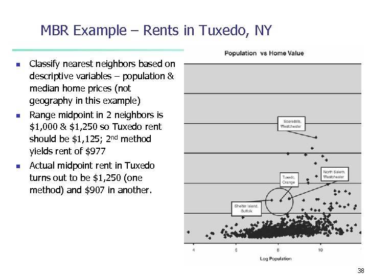MBR Example – Rents in Tuxedo, NY n n n Classify nearest neighbors based on descriptive variables – population & median home prices (not geography in this example) Range midpoint in 2 neighbors is $1, 000 & $1, 250 so Tuxedo rent should be $1, 125; 2 nd method yields rent of $977 Actual midpoint rent in Tuxedo turns out to be $1, 250 (one method) and $907 in another. 38

MBR Challenges 1. 2. 3. Choosing appropriate historical data for use in training Choosing the most efficient way to represent the training data Choosing the distance function, combination function, and the number of neighbors 39

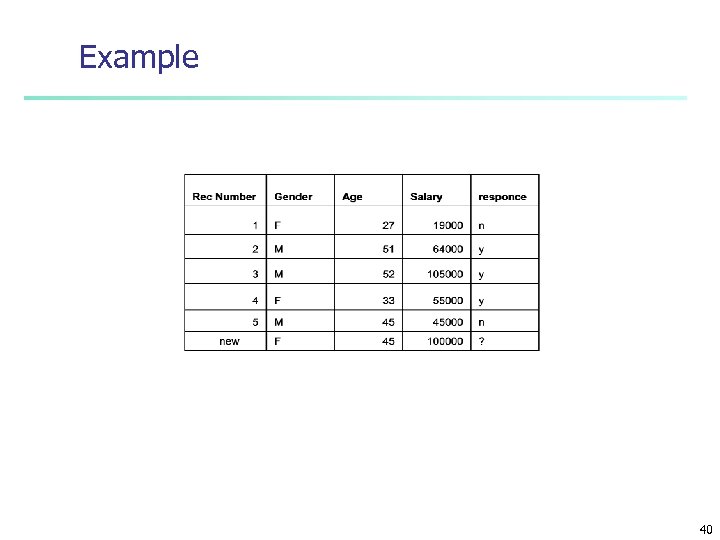Example 40

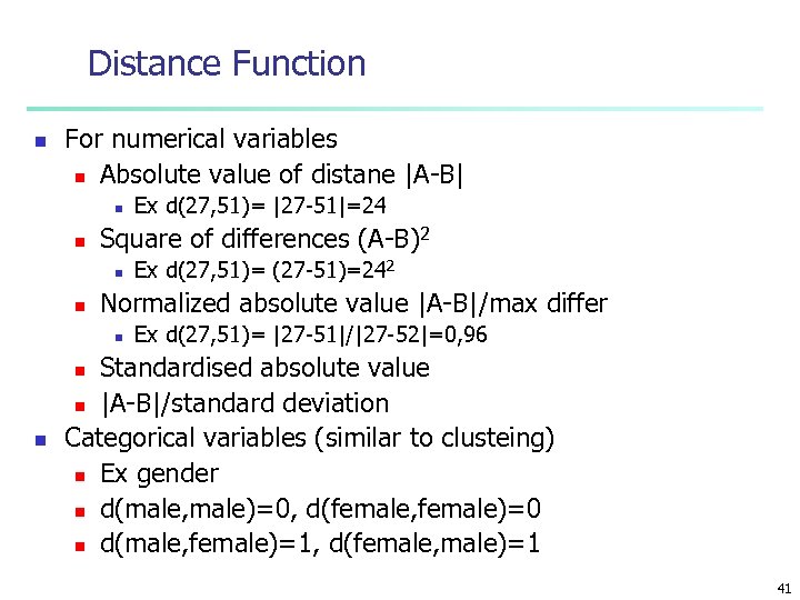Distance Function n For numerical variables n Absolute value of distane |A-B| n n Square of differences (A-B)2 n n Ex d(27, 51)= |27 -51|=24 Ex d(27, 51)= (27 -51)=242 Normalized absolute value |A-B|/max differ n Ex d(27, 51)= |27 -51|/|27 -52|=0, 96 Standardised absolute value n |A-B|/standard deviation Categorical variables (similar to clusteing) n Ex gender n d(male, male)=0, d(female, female)=0 n d(male, female)=1, d(female, male)=1 n n 41

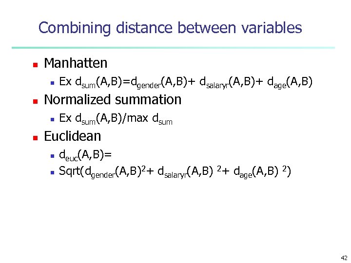Combining distance between variables n Manhatten n n Normalized summation n n Ex dsum(A, B)=dgender(A, B)+ dsalaryr(A, B)+ dage(A, B) Ex dsum(A, B)/max dsum Euclidean n n deuc(A, B)= Sqrt(dgender(A, B)2+ dsalaryr(A, B) 2+ dage(A, B) 2) 42

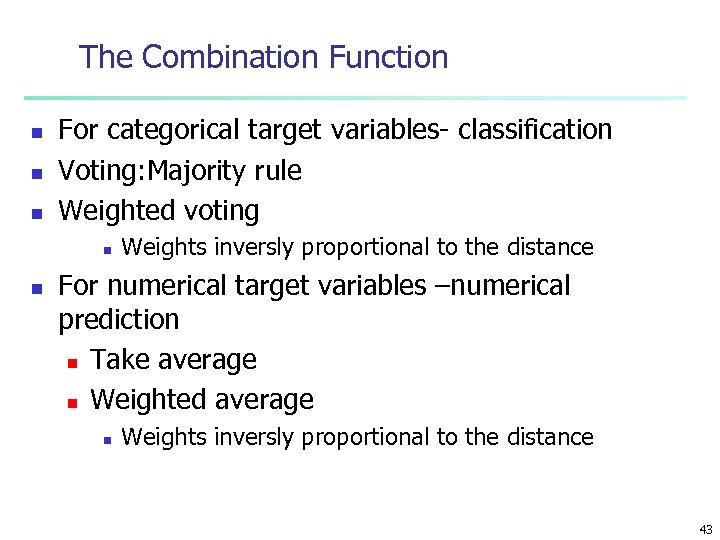The Combination Function n For categorical target variables- classification Voting: Majority rule Weighted voting n n Weights inversly proportional to the distance For numerical target variables –numerical prediction n Take average n Weighted average n Weights inversly proportional to the distance 43

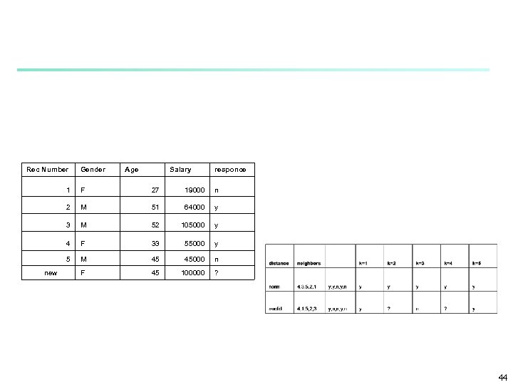Rec Number Gender Age Salary responce 1 27 19000 n 2 M 51 64000 y 3 M 52 105000 y 4 F 33 55000 y 5 new F M 45 45000 n F 45 100000 ? 44

Collaborative Filtering n n Lots of human examples of this: n Best teachers n Best courses n Best restaurants (ambiance, service, food, price) n Recommend a dentist, mechanic, PC repair, blank CDs/DVDs, wines, B&Bs, etc… CF is a variant of MBR particularly well suited to personalized recommendations 45

Collaborative Filtering n n Starts with a history of people’s personal preferences Uses a distance function – people who like the same things are “close” Uses “votes” which are weighted by distances, so close neighbor votes count more Basically, judgments of a peer group are important 46

Collaborative Filtering n n n Knowing that lots of people liked something is not sufficient… Who liked it is also important n Friend whose past recommendations were good (or bad) n High profile person seems to influence Collaborative Filtering automates this word-ofmouth everyday activity 47

Preparing Recommendations for Collaborative Filtering 1. 2. 3. Building customer profile – ask new customer to rate selection of things Comparing this new profile to other customers using some measure of similarity Using some combination of the ratings from similar customers to predict what the new customer would select for items he/she has NOT yet rated 48

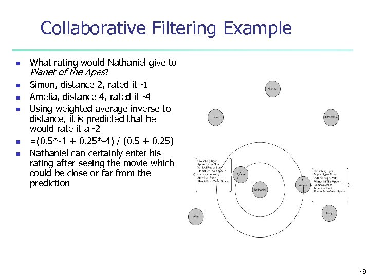Collaborative Filtering Example n n n What rating would Nathaniel give to Planet of the Apes? Simon, distance 2, rated it -1 Amelia, distance 4, rated it -4 Using weighted average inverse to distance, it is predicted that he would rate it a -2 =(0. 5*-1 + 0. 25*-4) / (0. 5 + 0. 25) Nathaniel can certainly enter his rating after seeing the movie which could be close or far from the prediction 49

Chapter 7. Classification and Prediction n n Bayesian Classification Model Based Reasoning Collaborative Filtering Classification accuracy 50

Holdout estimation n n What to do if the amount of data is limited? The holdout method reserves a certain amount for testing and uses the remainder for training n Usually: one third for testing, the rest for training Problem: the samples might not be representative n Example: class might be missing in the test data Advanced version uses stratification n Ensures that each class is represented with approximately equal proportions in both subsets 51

Repeated holdout method n n n Holdout estimate can be made more reliable by repeating the process with different subsamples n In each iteration, a certain proportion is randomly selected for training (possibly with stratificiation) n The error rates on the different iterations are averaged to yield an overall error rate This is called the repeated holdout method Still not optimum: the different test sets overlap n Can we prevent overlapping? 52

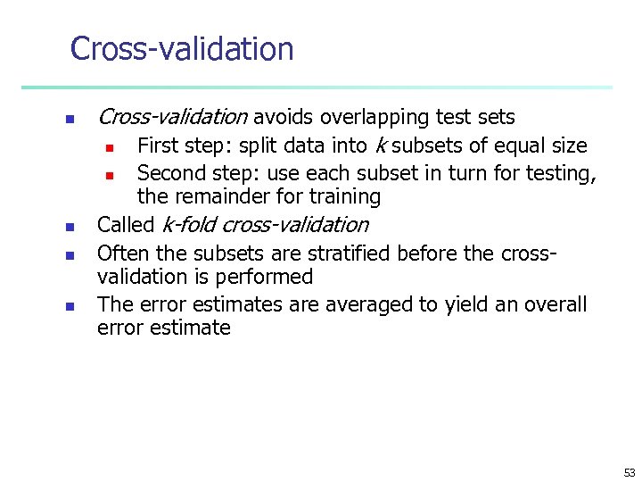Cross-validation n Cross-validation avoids overlapping test sets n First step: split data into k subsets of equal size Second step: use each subset in turn for testing, the remainder for training Called k-fold cross-validation Often the subsets are stratified before the crossvalidation is performed The error estimates are averaged to yield an overall error estimate n n 53

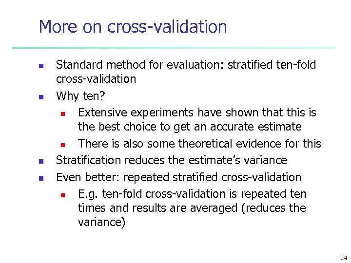More on cross-validation n n Standard method for evaluation: stratified ten-fold cross-validation Why ten? n Extensive experiments have shown that this is the best choice to get an accurate estimate n There is also some theoretical evidence for this Stratification reduces the estimate’s variance Even better: repeated stratified cross-validation n E. g. ten-fold cross-validation is repeated ten times and results are averaged (reduces the variance) 54

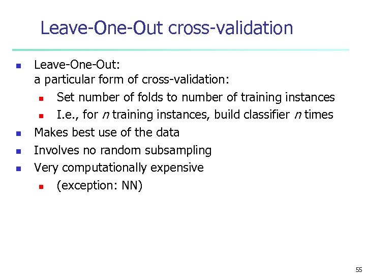Leave-One-Out cross-validation n n Leave-One-Out: a particular form of cross-validation: n Set number of folds to number of training instances n I. e. , for n training instances, build classifier n times Makes best use of the data Involves no random subsampling Very computationally expensive n (exception: NN) 55

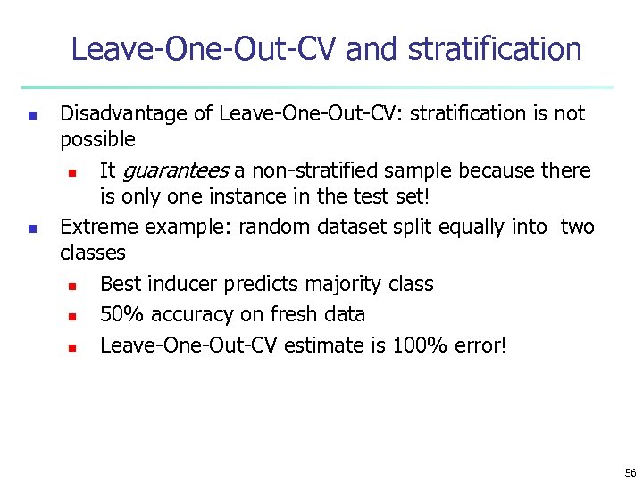Leave-One-Out-CV and stratification n n Disadvantage of Leave-One-Out-CV: stratification is not possible n It guarantees a non-stratified sample because there is only one instance in the test set! Extreme example: random dataset split equally into two classes n Best inducer predicts majority class n 50% accuracy on fresh data n Leave-One-Out-CV estimate is 100% error! 56

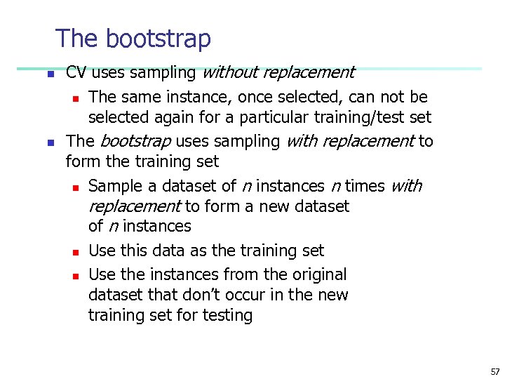The bootstrap n n CV uses sampling without replacement n The same instance, once selected, can not be selected again for a particular training/test set The bootstrap uses sampling with replacement to form the training set n Sample a dataset of n instances n times with replacement to form a new dataset of n instances n Use this data as the training set n Use the instances from the original dataset that don’t occur in the new training set for testing 57

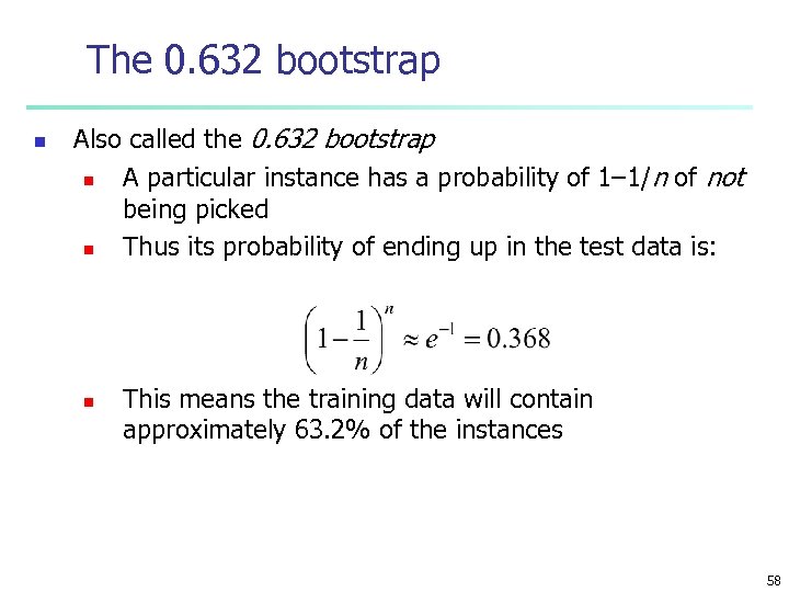The 0. 632 bootstrap n Also called the 0. 632 bootstrap n A particular instance has a probability of 1– 1/n of not being picked n Thus its probability of ending up in the test data is: n This means the training data will contain approximately 63. 2% of the instances 58

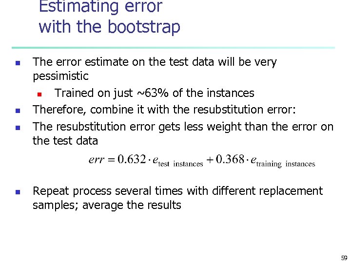Estimating error with the bootstrap n n The error estimate on the test data will be very pessimistic n Trained on just ~63% of the instances Therefore, combine it with the resubstitution error: The resubstitution error gets less weight than the error on the test data Repeat process several times with different replacement samples; average the results 59

Is accuracy enough to judge a classifier? n n Speed robustness (accuracy on noisy data) scalability n number of I/O opp. For large datasets interpretability n subjective n objective: n n number of hidden units for ANN number of tree notes for decision trees 60

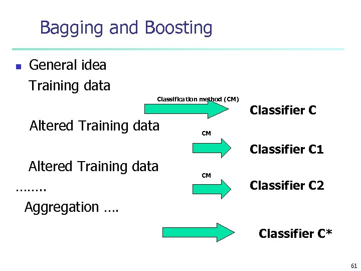Bagging and Boosting n General idea Training data Classification method (CM) Altered Training data Classifier C CM Classifier C 1 Altered Training data ……. . Aggregation …. CM Classifier C 2 Classifier C* 61

Bagging n n n Given a set S of s samples Generate a bootstrap sample T from S. Cases in S may not appear in T or may appear more than once. Repeat this sampling procedure, getting a sequence of k independent training sets A corresponding sequence of classifiers C 1, C 2, …, Ck is constructed for each of these training sets, by using the same classification algorithm To classify an unknown sample X, let each classifier predict or vote The Bagged Classifier C* counts the votes and assigns X to the class with the “most” votes 62

Increasing classifier accuracy-Bagging WF pp 250 -253 n n n n Bagging take t samples from data S sampling with replacement n each case may occur more than ones a new classifier Ct is learned for each set St Form the bagged classifier C* by voting classifiers equally n the majority rule For continuous valued prediction problems n take the average of each predictor 63

Increasing classifier accuracy. Boosting WF pp 254 -258 n n n Boosting increases classification accuracy n Applicable to decision trees or Bayesian classifier Learn a series of classifiers, where each classifier in the series pays more attention to the examples misclassified by its predecessor Boosting requires only linear time and constant space 64

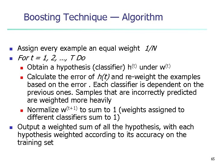Boosting Technique — Algorithm n Assign every example an equal weight 1/N n For t = 1, 2, …, T Do Obtain a hypothesis (classifier) h(t) under w(t) n Calculate the error of h(t) and re-weight the examples based on the error. Each classifier is dependent on the previous ones. Samples that are incorrectly predicted are weighted more heavily (t+1) to sum to 1 (weights assigned to n Normalize w different classifiers sum to 1) Output a weighted sum of all the hypothesis, with each hypothesis weighted according to its accuracy on the training set n n 65

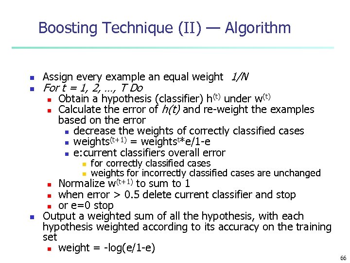Boosting Technique (II) — Algorithm n n Assign every example an equal weight 1/N For t = 1, 2, …, T Do n n Obtain a hypothesis (classifier) h(t) under w(t) Calculate the error of h(t) and re-weight the examples based on the error n decrease the weights of correctly classified cases (t+1) = weightst*e/1 -e n weights n e: current classifiers overall error n n for correctly classified cases weights for incorrectly classified cases are unchanged Normalize w(t+1) to sum to 1 n when error > 0. 5 delete current classifier and stop n or e=0 stop Output a weighted sum of all the hypothesis, with each hypothesis weighted according to its accuracy on the training set n weight = -log(e/1 -e) n n 66

Bagging and Boosting n n n Experiments with a new boosting algorithm, freund et al (Ada. Boost ) Bagging Predictors, Brieman Boosting Naïve Bayesian Learning on large subset of MEDLINE, W. Wilbur 67

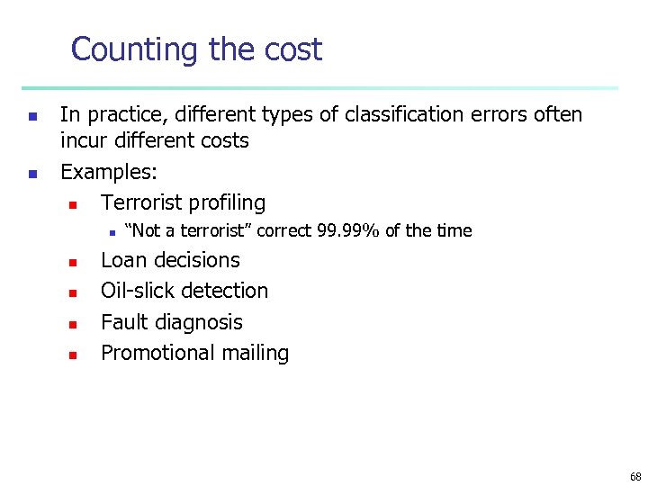Counting the cost n n In practice, different types of classification errors often incur different costs Examples: n Terrorist profiling n n n “Not a terrorist” correct 99. 99% of the time Loan decisions Oil-slick detection Fault diagnosis Promotional mailing 68

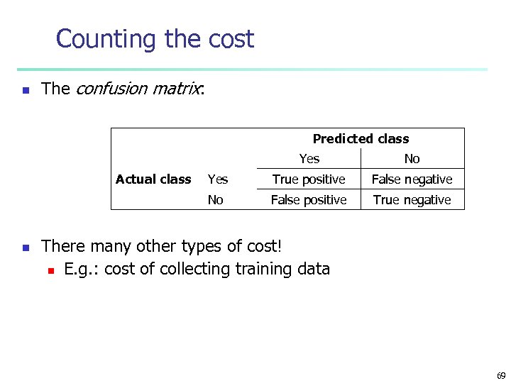Counting the cost n The confusion matrix: Predicted class Yes n Yes True positive False negative No Actual class No False positive True negative There many other types of cost! n E. g. : cost of collecting training data 69

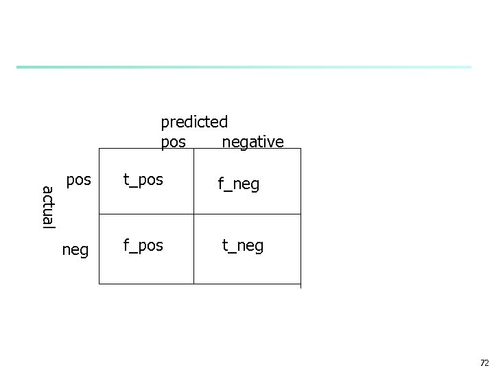
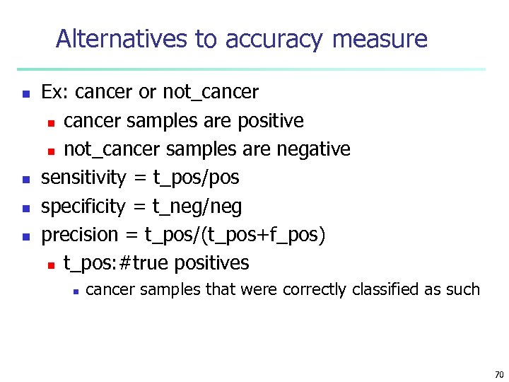Alternatives to accuracy measure n n Ex: cancer or not_cancer n cancer samples are positive n not_cancer samples are negative sensitivity = t_pos/pos specificity = t_neg/neg precision = t_pos/(t_pos+f_pos) n t_pos: #true positives n cancer samples that were correctly classified as such 70

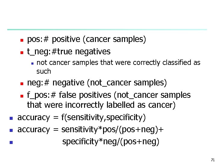n n pos: # positive (cancer samples) t_neg: #true negatives n not cancer samples that were correctly classified as such neg: # negative (not_cancer samples) n f_pos: # false positives (not_cancer samples that were incorrectly labelled as cancer) accuracy = f(sensitivity, specificity) accuracy = sensitivity*pos/(pos+neg)+ specificity*neg/(pos+neg) n n 71

predicted pos negative actual pos t_pos f_neg f_pos t_neg 72

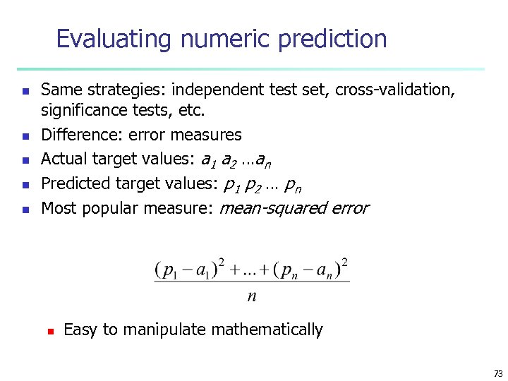Evaluating numeric prediction n n Same strategies: independent test set, cross-validation, significance tests, etc. Difference: error measures Actual target values: a 1 a 2 …an Predicted target values: p 1 p 2 … pn Most popular measure: mean-squared error n Easy to manipulate mathematically 73

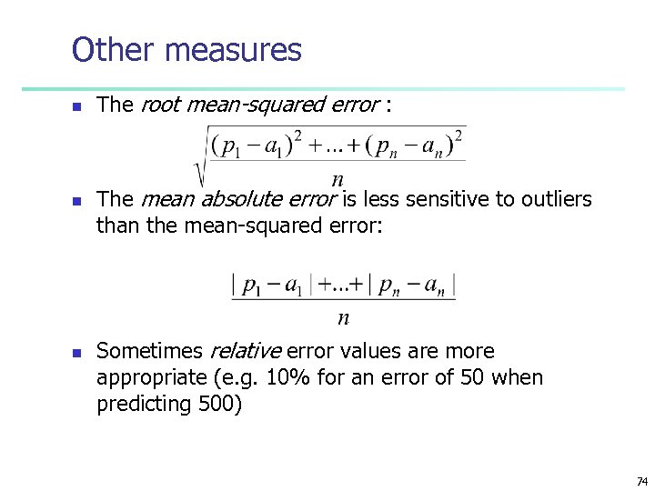Other measures n n n The root mean-squared error : The mean absolute error is less sensitive to outliers than the mean-squared error: Sometimes relative error values are more appropriate (e. g. 10% for an error of 50 when predicting 500) 74

Lift charts n n n In practice, costs are rarely known Decisions are usually made by comparing possible scenarios Example: promotional mailout to 1, 000 households • Mail to all; 0. 1% respond (1000) • Data mining tool identifies subset of 100, 000 most promising, 0. 4% of these respond (400) 40% of responses for 10% of cost may pay off Identify subset of 400, 000 most promising, 0. 2% respond (800) A lift chart allows a visual comparison • n 75

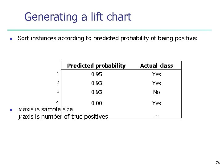Generating a lift chart n Sort instances according to predicted probability of being positive: Predicted probability 1 0. 95 Yes 2 0. 93 Yes 3 0. 93 No 4 n Actual class 0. 88 Yes x axis is sample size … … y axis is number of true positives … 76

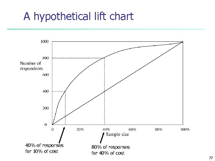A hypothetical lift chart 40% of responses for 10% of cost 80% of responses for 40% of cost 77

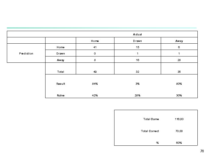Actual Home Drawn Away Home 41 15 6 Prediction Drawn 0 1 1 Away 8 16 28 Total 49 32 35 Result 84% 3% 80% Naïve 42% 28% 30% Total Game 116, 00 Total Correct 70, 00 % 60% 78

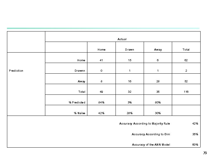Actual Home Drawn Away Total Home 41 15 6 62 Drawnn 0 1 1 2 Away 8 16 28 52 Total 49 32 35 116 % Predicted 84% 3% 80% % Naïve 42% 28% 30% Prediction Accuracy According to Majority Rule 42% Accuracy According to Gini 35% Accuracy of the ANN Model 60% 79