8a42e9f8878d5abeef0048c800fed603.ppt
- Количество слайдов: 136
 Data Mining Algorithms for Recommendation Systems Zhenglu Yang University of Tokyo Some slides are from online materials.
 Applications 2
 Applications 3
 Applications Corporate Intranets 4
 System Inputs o Interaction data (users items) n Explicit feedback – rating, comments n Implicit feedback – purchase, browsing o User/Item individual data n User side: o Structural attribute information o Personal description o Social network n Item side: o Structural attribute information o Textual description/content information o Taxonomy of item (category) 5
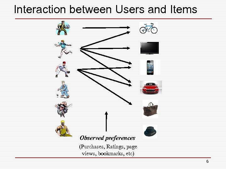 Interaction between Users and Items Observed preferences (Purchases, Ratings, page views, bookmarks, etc) 6
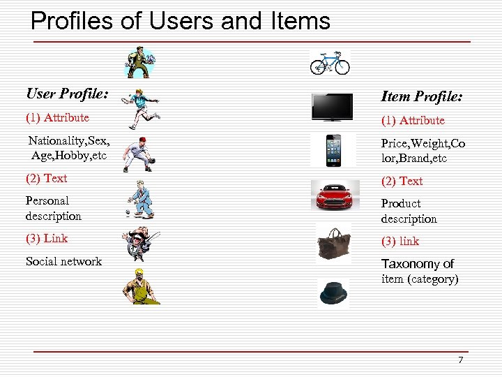 Profiles of Users and Items User Profile: Item Profile: (1) Attribute Nationality, Sex, Age, Hobby, etc Price, Weight, Co lor, Brand, etc (2) Text Personal description Product description (3) Link (3) link Social network Taxonomy of item (category) 7
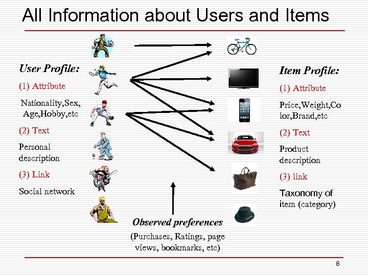 All Information about Users and Items User Profile: Item Profile: (1) Attribute Nationality, Sex, Age, Hobby, etc Price, Weight, Co lor, Brand, etc (2) Text Personal description Product description (3) Link (3) link Social network Taxonomy of item (category) Observed preferences (Purchases, Ratings, page views, bookmarks, etc) 8
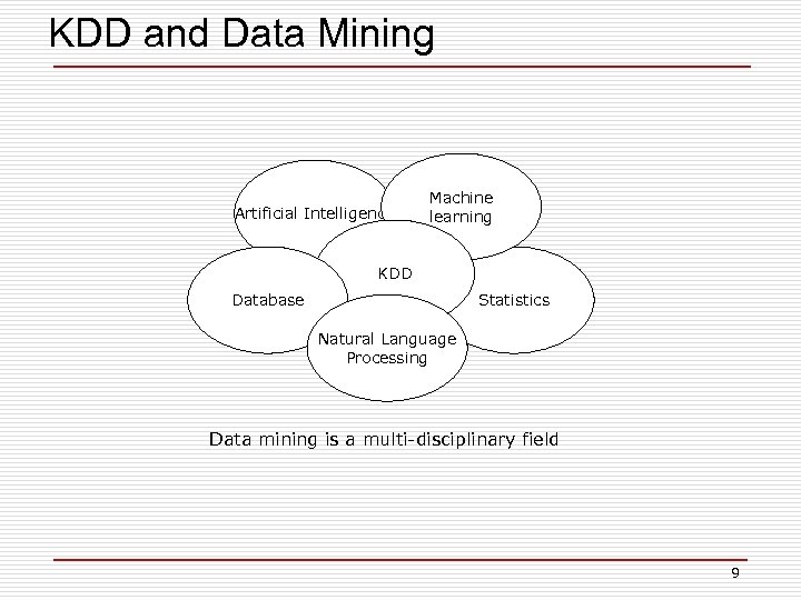 KDD and Data Mining Artificial Intelligence Machine learning KDD Database Statistics Natural Language Processing Data mining is a multi-disciplinary field 9
 Recommendation Approaches o Collaborative filtering n Using interaction data (user-item matrix) n Process: Identify similar users, extrapolate from their ratings o Content based strategies n Using profiles of users/items (features) n Process: Generate rules/classifiers that are used to classify new items o Hybrid approaches 10
 A Brief Introduction o Collaborative filtering n Nearest neighbor based n Model based 11
 Recommendation Approaches o Collaborative filtering n Nearest neighbor based o User based o Item based n Model based 12
 User-based Collaborative Filtering o Idea: people who agreed in the past are likely to agree again o To predict a user’s opinion for an item, use the opinion of similar users o Similarity between users is decided by looking at their overlap in opinions for other items
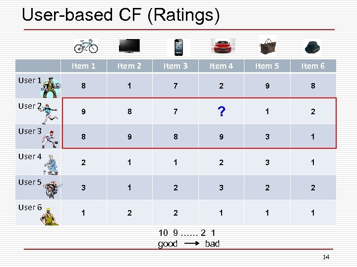 User-based CF (Ratings) Item 1 User 2 User 3 User 4 User 5 User 6 Item 2 Item 3 Item 4 Item 5 Item 6 8 1 7 2 9 8 7 ? 1 2 8 9 3 1 2 1 1 2 3 2 2 1 1 1 10 9 …… 2 1 good bad 14
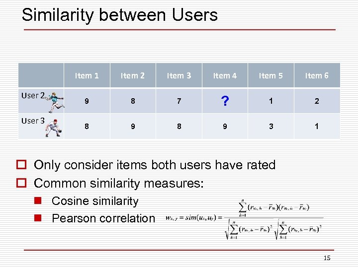 Similarity between Users Item 1 User 2 User 3 Item 2 Item 3 Item 4 Item 5 Item 6 9 8 7 ? 1 2 8 9 3 1 o Only consider items both users have rated o Common similarity measures: n Cosine similarity n Pearson correlation 15
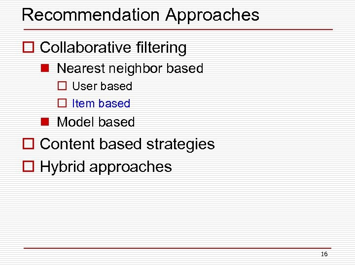 Recommendation Approaches o Collaborative filtering n Nearest neighbor based o User based o Item based n Model based o Content based strategies o Hybrid approaches 16
 Item-based Collaborative Filtering o Idea: a user is likely to have the same opinion for similar items o Similarity between items is decided by looking at how other users have rated them 17
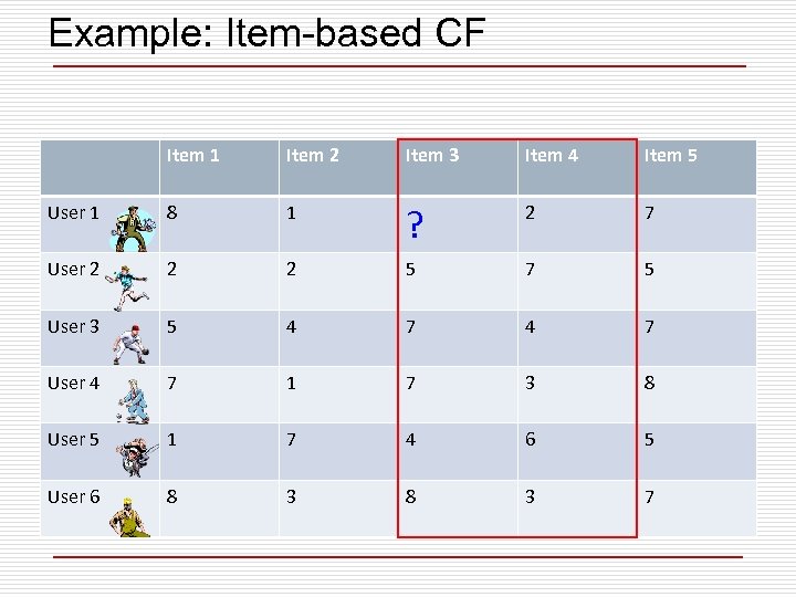 Example: Item-based CF Item 1 Item 2 Item 3 Item 4 Item 5 User 1 8 1 ? 2 7 User 2 2 2 5 7 5 User 3 5 4 7 User 4 7 1 7 3 8 User 5 1 7 4 6 5 User 6 8 3 7
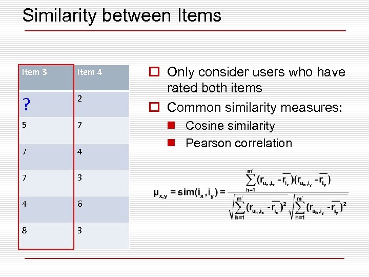 Similarity between Items Item 3 Item 4 ? 2 5 7 7 4 7 3 4 6 8 3 o Only consider users who have rated both items o Common similarity measures: n Cosine similarity n Pearson correlation
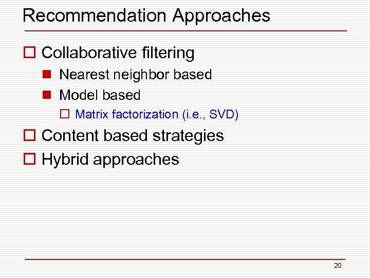 Recommendation Approaches o Collaborative filtering n Nearest neighbor based n Model based o Matrix factorization (i. e. , SVD) o Content based strategies o Hybrid approaches 20
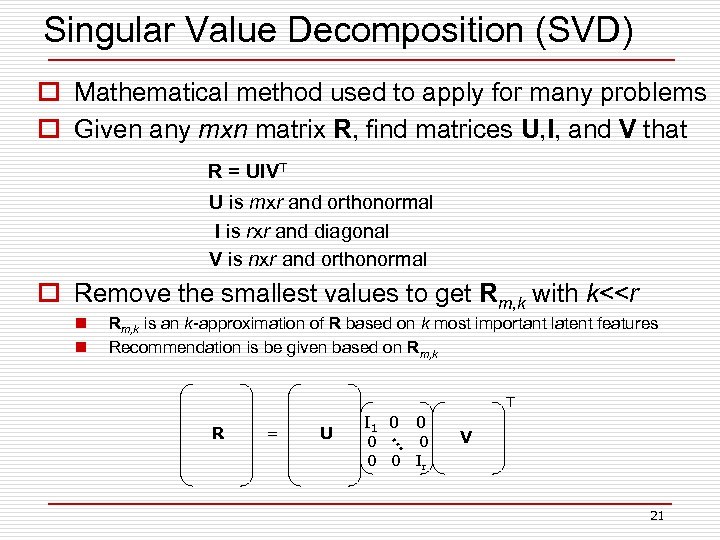 Singular Value Decomposition (SVD) o Mathematical method used to apply for many problems o Given any mxn matrix R, find matrices U, I, and V that R = UIVT U is mxr and orthonormal I is rxr and diagonal V is nxr and orthonormal o Remove the smallest values to get Rm, k with k<
 Problems with Collaborative Filtering o Cold Start: There needs to be enough other users already in the system to find a match. o Sparsity: If there are many items to be recommended, even if there are many users, the user/ratings matrix is sparse, and it is hard to find users that have rated the same items. o First Rater: Cannot recommend an item that has not been previously rated. n New items n Esoteric items o Popularity Bias: Cannot recommend items to someone with unique tastes. n Tends to recommend popular items. 22
 Recommendation Approaches o Collaborative filtering o Content based strategies o Hybrid approaches 23
 Profiles of Users and Items User Profile: Item Profile: (1) Attribute Nationality, Sex, Age, Hobby, etc Price, Weight, Co lor, Brand, etc (2) Text Personal description Product description (3) Link (3) link Social network Taxonomy of item (category) 24
 Advantages of Content-Based Approach o No need for data on other users. n No cold-start or sparsity problems. o Able to recommend to users with unique tastes. o Able to recommend new and unpopular items n No first-rater problem. o Can provide explanations of recommended items by listing content-features that caused an item to be recommended. 25
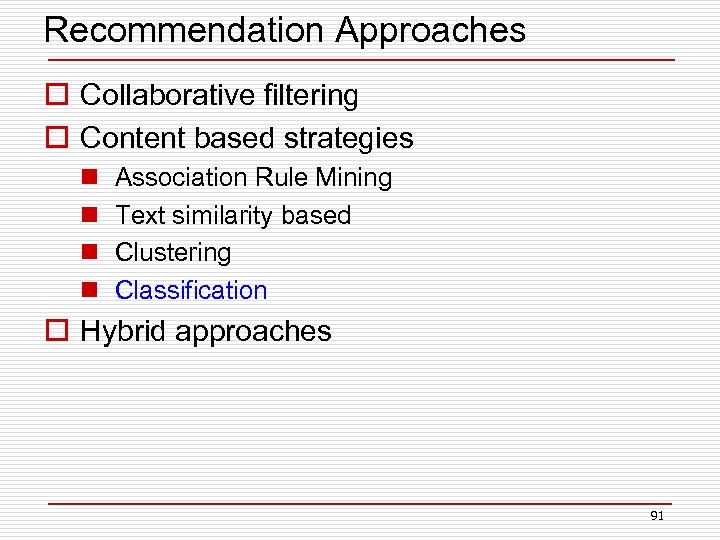
 Recommendation Approaches o Collaborative filtering o Content based strategies n n Association Rule Mining Text similarity based Clustering Classification o Hybrid approaches 26
 Traditional Data Mining Techniques o Association Rule Mining (ARM) o Sequential Pattern Mining (SPM) 27
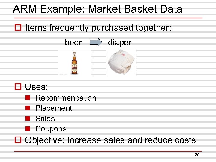 ARM Example: Market Basket Data o Items frequently purchased together: beer diaper o Uses: n n Recommendation Placement Sales Coupons o Objective: increase sales and reduce costs 28
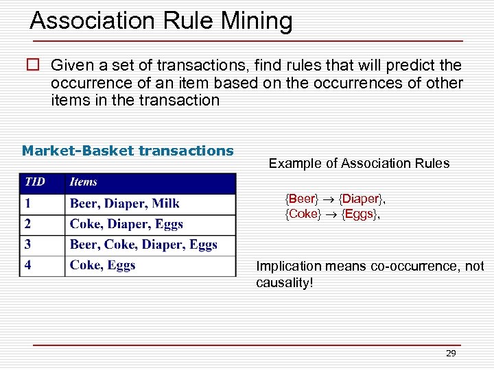 Association Rule Mining o Given a set of transactions, find rules that will predict the occurrence of an item based on the occurrences of other items in the transaction Market-Basket transactions Example of Association Rules {Beer} {Diaper}, {Coke} {Eggs}, Implication means co-occurrence, not causality! 29
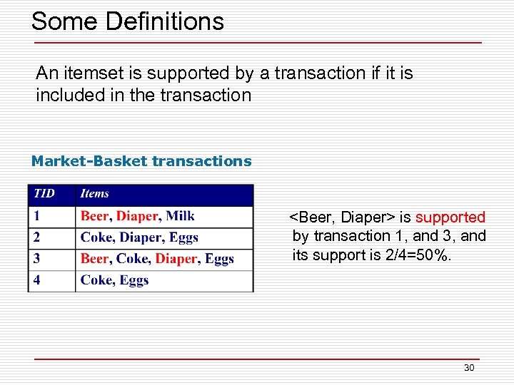 Some Definitions An itemset is supported by a transaction if it is included in the transaction Market-Basket transactions
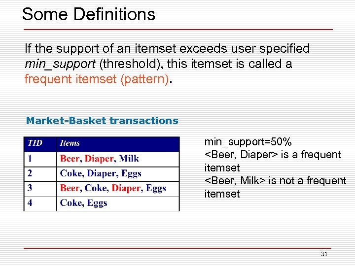 Some Definitions If the support of an itemset exceeds user specified min_support (threshold), this itemset is called a frequent itemset (pattern). Market-Basket transactions min_support=50%
 Outline o Association Rule Mining n Apriori n FP-growth o Sequential Pattern Mining 32
![Apriori Algorithm o Proposed by Agrawal et al. [VLDB’ 94] o First algorithm for Apriori Algorithm o Proposed by Agrawal et al. [VLDB’ 94] o First algorithm for](https://present5.com/presentation/8a42e9f8878d5abeef0048c800fed603/image-33.jpg) Apriori Algorithm o Proposed by Agrawal et al. [VLDB’ 94] o First algorithm for Association Rule mining o Candidate generation-and-test o Introduced anti-monotone property 33
Apriori Algorithm o Proposed by Agrawal et al. [VLDB’ 94] o First algorithm for Association Rule mining o Candidate generation-and-test o Introduced anti-monotone property 33
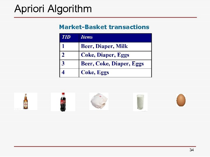 Apriori Algorithm Market-Basket transactions 34
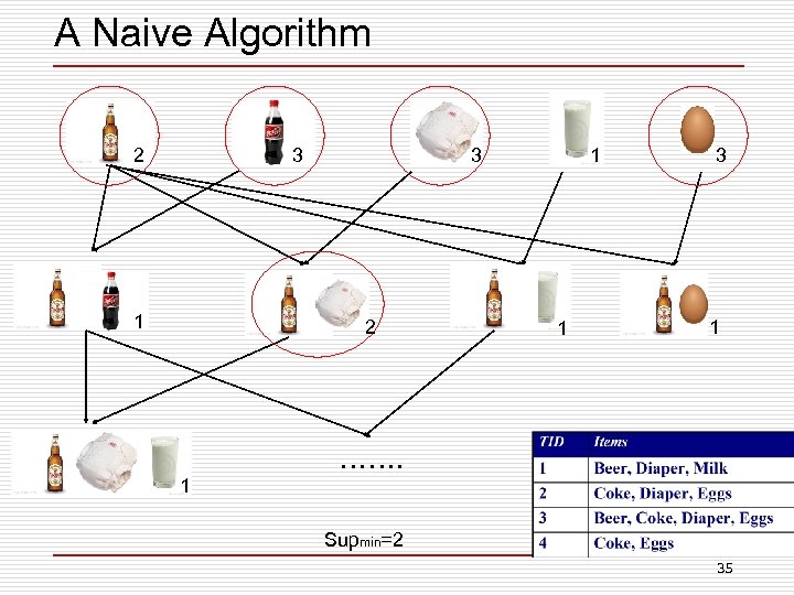 A Naive Algorithm 2 3 12 1 1 3 1 ……. 1 Supmin=2 35
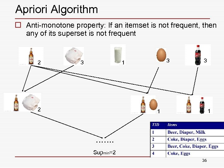 Apriori Algorithm o Anti-monotone property: If an itemset is not frequent, then any of its superset is not frequent 2 3 3 1 2 3 1 1 ……. Supmin=2 36
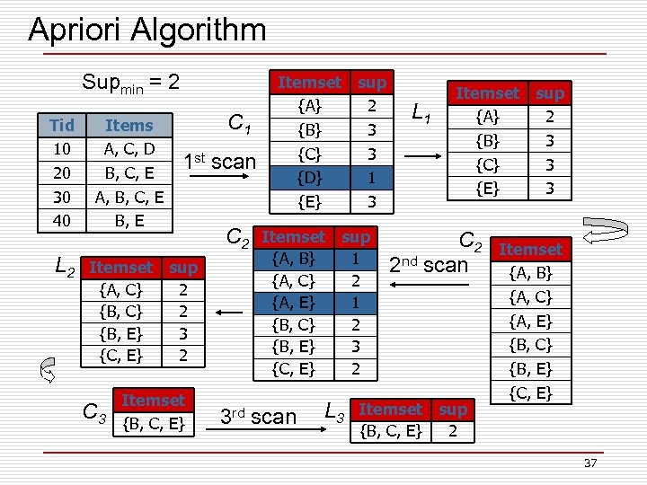 Apriori Algorithm Supmin = 2 Tid 10 20 30 40 L 2 Items A, C, D B, C, E A, B, C, E B, E C 1 1 st scan Itemset sup {A, C} 2 {B, E} 3 {C, E} 2 Itemset C 3 {B, C, E} C 2 Itemset sup {A} 2 {B} 3 {C} 3 {D} 1 {E} 3 Itemset sup {A, B} 1 {A, C} 2 {A, E} 1 {B, C} 2 {B, E} 3 {C, E} 2 3 rd scan L 3 L 1 Itemset sup {A} 2 {B} 3 {C} 3 {E} 3 C 2 2 nd scan Itemset sup {B, C, E} 2 Itemset {A, B} {A, C} {A, E} {B, C} {B, E} {C, E} 37
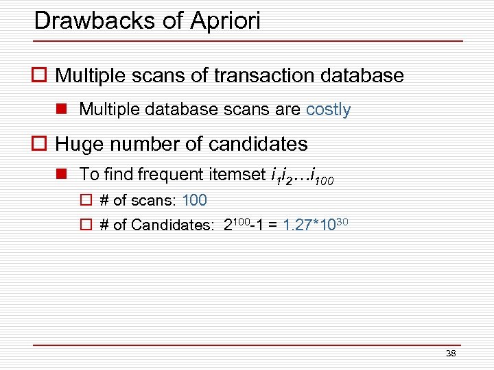 Drawbacks of Apriori o Multiple scans of transaction database n Multiple database scans are costly o Huge number of candidates n To find frequent itemset i 1 i 2…i 100 o # of scans: 100 o # of Candidates: 2100 -1 = 1. 27*1030 38
 Outline o Association Rule Mining n Apriori n FP-growth o Sequential Pattern Mining 39
![FP-Growth o Proposed by Han et al. [SIGMOD’ 00] o Uses the Apriori pruning FP-Growth o Proposed by Han et al. [SIGMOD’ 00] o Uses the Apriori pruning](https://present5.com/presentation/8a42e9f8878d5abeef0048c800fed603/image-40.jpg) FP-Growth o Proposed by Han et al. [SIGMOD’ 00] o Uses the Apriori pruning principle o Scan DB only twice n Once to find frequent 1 -itemset (single item pattern) n Once to construct FP-tree (prefix tree, Trie), the data structure of FP-growth 40
FP-Growth o Proposed by Han et al. [SIGMOD’ 00] o Uses the Apriori pruning principle o Scan DB only twice n Once to find frequent 1 -itemset (single item pattern) n Once to construct FP-tree (prefix tree, Trie), the data structure of FP-growth 40
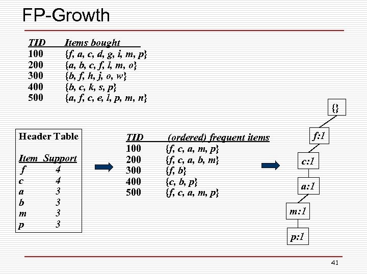 FP-Growth TID 100 200 300 400 500 Items bought {f, a, c, d, g, i, m, p} {a, b, c, f, l, m, o} {b, f, h, j, o, w} {b, c, k, s, p} {a, f, c, e, l, p, m, n} Header Table Item Support f 4 c 4 a 3 b 3 m 3 p 3 TID 100 200 300 400 500 {} (ordered) frequent items {f, c, a, m, p} {f, c, a, b, m} {f, b} {c, b, p} {f, c, a, m, p} f: 1 c: 1 a: 1 m: 1 p: 1 41
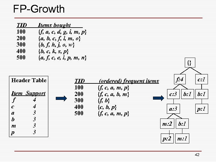 FP-Growth TID 100 200 300 400 500 Items bought {f, a, c, d, g, i, m, p} {a, b, c, f, l, m, o} {b, f, h, j, o, w} {b, c, k, s, p} {a, f, c, e, l, p, m, n} Header Table Item Support f 4 c 4 a 3 b 3 m 3 p 3 TID 100 200 300 400 500 {} (ordered) frequent items {f, c, a, m, p} {f, c, a, b, m} {f, b} {c, b, p} {f, c, a, m, p} f: 4 c: 3 c: 1 b: 1 a: 3 b: 1 p: 1 m: 2 b: 1 p: 2 m: 1 42
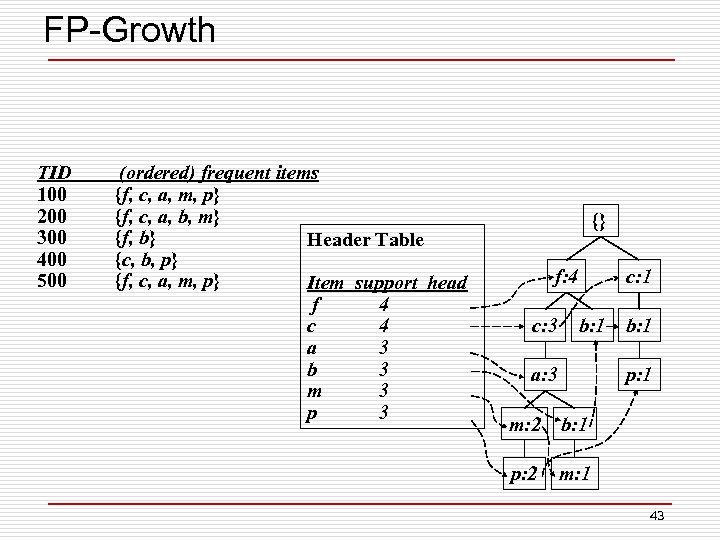 FP-Growth TID 100 200 300 400 500 (ordered) frequent items {f, c, a, m, p} {f, c, a, b, m} {f, b} Header Table {c, b, p} {f, c, a, m, p} Item support head f 4 c 4 a 3 b 3 m 3 p 3 {} f: 4 c: 3 c: 1 b: 1 a: 3 b: 1 p: 1 m: 2 b: 1 p: 2 m: 1 43
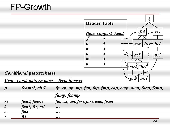 FP-Growth {} Header Table Item support head f 4 c 4 a 3 b 3 m 3 p 3 Conditional pattern bases Item cond. pattern base p fcam: 2, cb: 1 freq. itemset f: 4 c: 1 c: 3 b: 1 a: 3 p: 1 m: 2 b: 1 p: 2 m: 1 fp, cp, ap, mp, fcp, fap, fmp, cap, cmp, amp, facp, fcmp, famp, fcamp m b a c fca: 2, fcab: 1 fca: 1, f: 1, c: 1 fc: 3 fm, cm, am, fcm, fam, cam, fcam … … … 44
 Outline o Association Rule Mining n Apriori n FP-growth o Sequential Pattern Mining n GSP n SPADE, SPAM n Prefix. Span 45
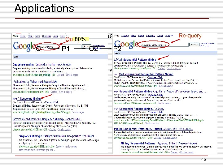 Applications o Customer shopping sequences Query 80% Q 1 P 1 Note computer Q 2 Re-query P 2 Memory CD-ROM within 3 days 46
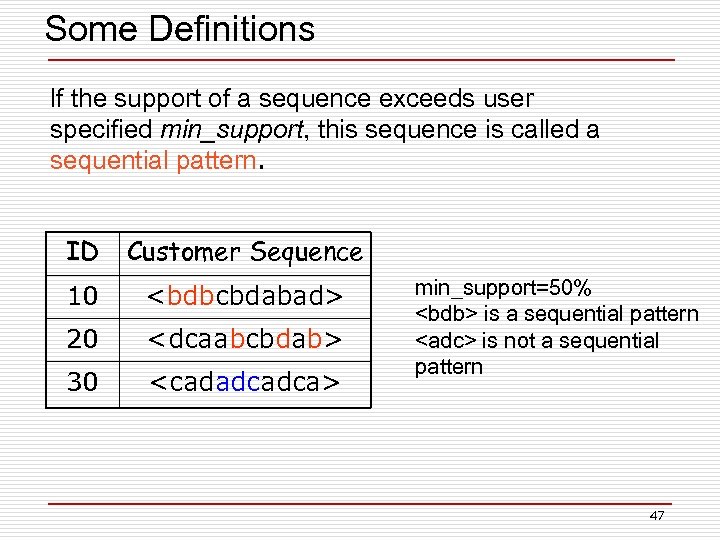 Some Definitions If the support of a sequence exceeds user specified min_support, this sequence is called a sequential pattern. ID Customer Sequence 10
 Outline o Association Rule Mining n Apriori n FP-growth o Sequential Pattern Mining n GSP n SPADE, SPAM n Prefix. Span 48
![GSP (Generalized Sequential Pattern Mining) o Proposed by Srikant et al. [EDBT’ 96] o GSP (Generalized Sequential Pattern Mining) o Proposed by Srikant et al. [EDBT’ 96] o](https://present5.com/presentation/8a42e9f8878d5abeef0048c800fed603/image-49.jpg) GSP (Generalized Sequential Pattern Mining) o Proposed by Srikant et al. [EDBT’ 96] o Uses the Apriori pruning principle o Outline of the method n Initially, every item in DB is a candidate of length-1 n For each level (i. e. , sequences of length-k) do o Scan database to collect support count for each candidate sequence o Generate candidate length-(k+1) sequences from length-k frequent sequences using Apriori n Repeat until no frequent sequence or no candidate can be found 49
GSP (Generalized Sequential Pattern Mining) o Proposed by Srikant et al. [EDBT’ 96] o Uses the Apriori pruning principle o Outline of the method n Initially, every item in DB is a candidate of length-1 n For each level (i. e. , sequences of length-k) do o Scan database to collect support count for each candidate sequence o Generate candidate length-(k+1) sequences from length-k frequent sequences using Apriori n Repeat until no frequent sequence or no candidate can be found 49
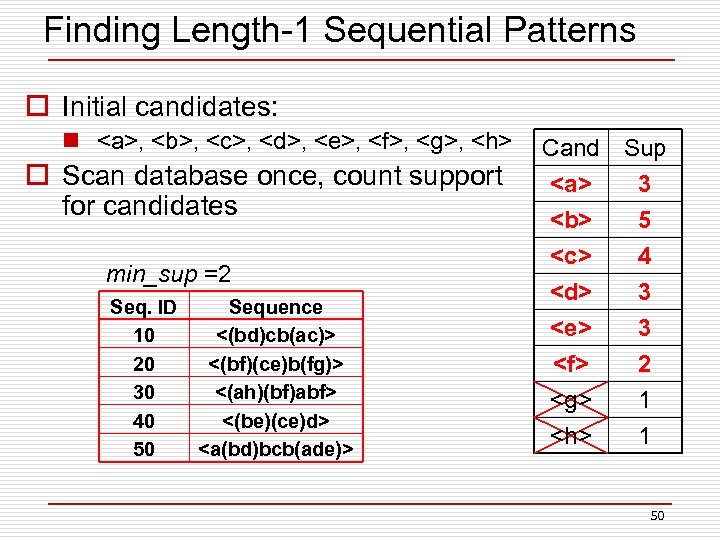 Finding Length-1 Sequential Patterns o Initial candidates: n , ,
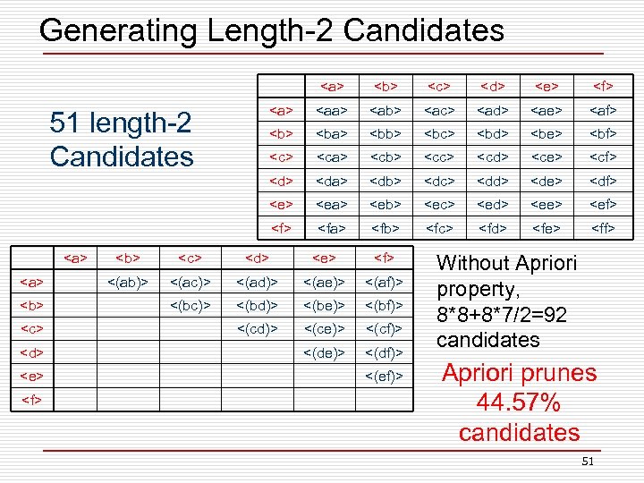 Generating Length-2 Candidates
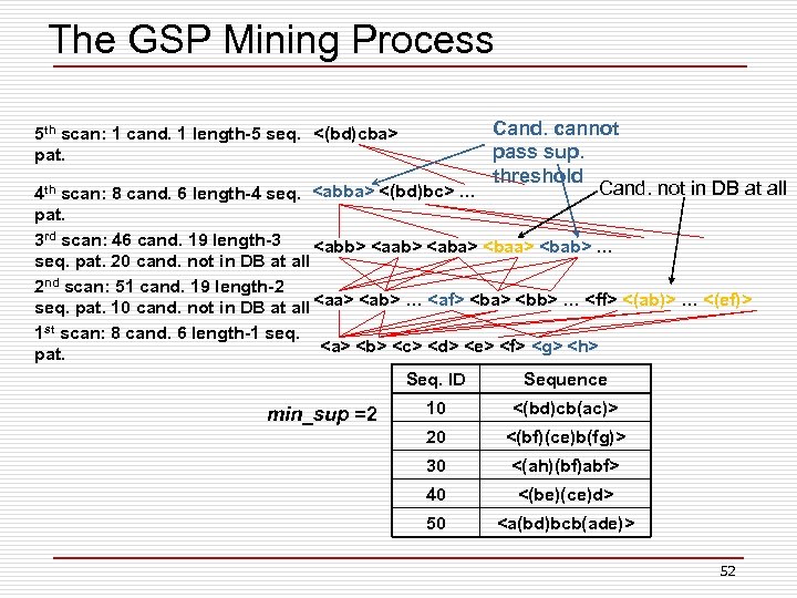 The GSP Mining Process Cand. cannot pass sup. threshold Cand. not in DB at all 4 th scan: 8 cand. 6 length-4 seq.
 Outline o Association Rule Mining n Apriori n FP-growth o Sequential Pattern Mining n GSP n SPADE, SPAM n Prefix. Span 53
![SPADE Algorithm o Proposed by Zaki et al. [MLJ’ 01] o Vertical ID-list data SPADE Algorithm o Proposed by Zaki et al. [MLJ’ 01] o Vertical ID-list data](https://present5.com/presentation/8a42e9f8878d5abeef0048c800fed603/image-54.jpg) SPADE Algorithm o Proposed by Zaki et al. [MLJ’ 01] o Vertical ID-list data representation o Support counting n Temporal joins o Candidate to be tested n In local candidate lists 54
SPADE Algorithm o Proposed by Zaki et al. [MLJ’ 01] o Vertical ID-list data representation o Support counting n Temporal joins o Candidate to be tested n In local candidate lists 54
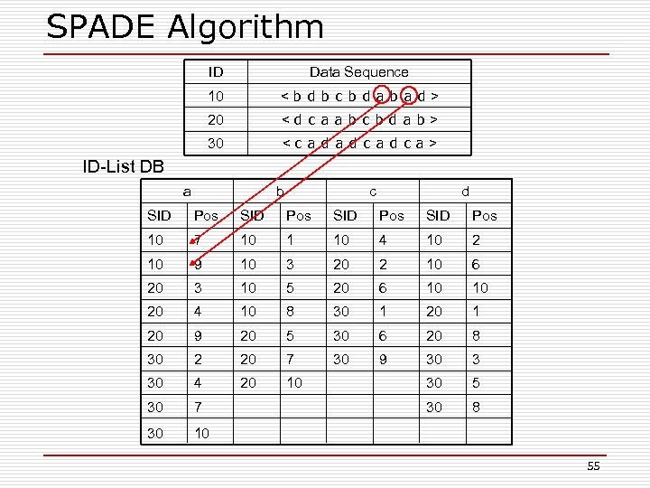 SPADE Algorithm ID Data Sequence 10 < b d b c b d a b a d > 20 < d c a a b c b d a b > 30 < c a d c a > ID-List DB a b c d SID Pos 10 7 10 1 10 4 10 2 10 9 10 3 20 2 10 6 20 3 10 5 20 6 10 10 20 4 10 8 30 1 20 9 20 5 30 6 20 8 30 2 20 7 30 9 30 3 30 4 20 10 30 5 30 7 30 8 30 10 55
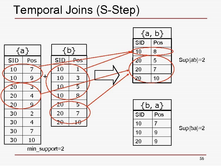 Temporal Joins (S-Step) {a, b} SID 10 {b} {a} Pos 8 SID Pos 20 5 10 7 10 1 20 7 10 9 10 3 20 10 20 3 10 5 20 4 10 8 20 9 20 5 30 2 20 7 SID Pos 30 4 20 10 10 7 30 7 10 9 30 10 20 9 + Sup{ab}=2 {b, a} Sup{ba}=2 min_support=2 56
 Outline o Association Rule Mining n Apriori n FP-growth o Sequential Pattern Mining n GSP n SPADE, SPAM n Prefix. Span 57
![SPAM Algorithm o Proposed by Ayres et al. [KDD’ 02] o Key idea based SPAM Algorithm o Proposed by Ayres et al. [KDD’ 02] o Key idea based](https://present5.com/presentation/8a42e9f8878d5abeef0048c800fed603/image-58.jpg) SPAM Algorithm o Proposed by Ayres et al. [KDD’ 02] o Key idea based on SPADE o Using bitmap data representation o Much faster than SPADE yet space consuming 58
SPAM Algorithm o Proposed by Ayres et al. [KDD’ 02] o Key idea based on SPADE o Using bitmap data representation o Much faster than SPADE yet space consuming 58
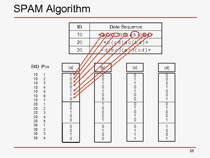 SPAM Algorithm ID 10 1 2 3 4 5 6 7 1 2 3 4 5 1 2 3 4
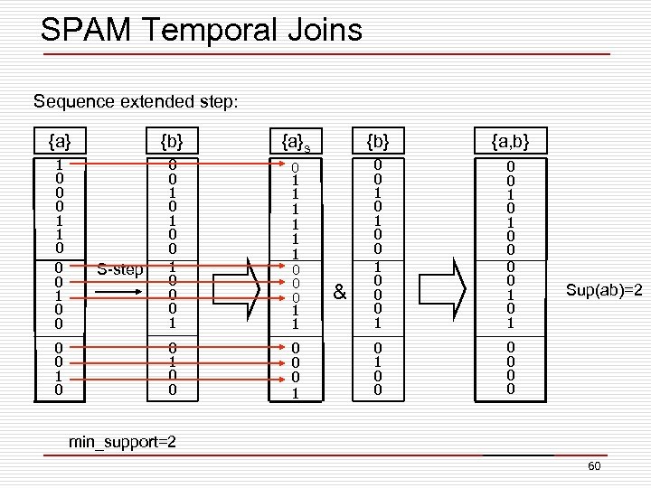 SPAM Temporal Joins Sequence extended step: {a} {b} {a}s {b} {a, b} 1 0 0 0 1 0 0 1 0 0 0 1 1 1 1 0 0 0 1 1 0 0 0 1 0 1 0 0 0 1 0 0 0 0 1 0 S-step & Sup(ab)=2 min_support=2 60
 Outline o Association Rule Mining n Apriori n FP-growth o Sequential Pattern Mining n GSP n SPADE, SPAM n Prefix. Span 61
![Prefix. Span (Projection-based Approach) o Proposed by Pei et al. [ICDE’ 01] o Based Prefix. Span (Projection-based Approach) o Proposed by Pei et al. [ICDE’ 01] o Based](https://present5.com/presentation/8a42e9f8878d5abeef0048c800fed603/image-62.jpg) Prefix. Span (Projection-based Approach) o Proposed by Pei et al. [ICDE’ 01] o Based on pattern growth o Prefix-Postfix (Projection) representation o Basic idea: use frequent items to recursively project sequence database into smaller projected databases and grow patterns in each projected database. 62
Prefix. Span (Projection-based Approach) o Proposed by Pei et al. [ICDE’ 01] o Based on pattern growth o Prefix-Postfix (Projection) representation o Basic idea: use frequent items to recursively project sequence database into smaller projected databases and grow patterns in each projected database. 62
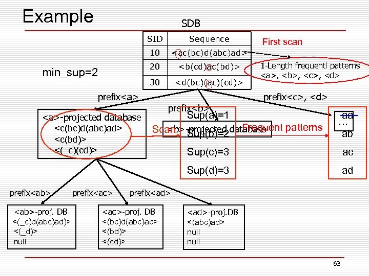 Example SDB SID 10
 Recommendation Approaches o Collaborative filtering o Content based strategies n n Association Rule Mining Text similarity based Clustering Classification o Hybrid approaches 64
 Text Similarity based Techniques o Vector Space Model (VSM) n TF-IDF o Semantic resource based n Wordnet n Wiki n Web 65
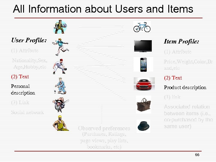 All Information about Users and Items User Profile: Item Profile: (1) Attribute Nationality, Sex, Age, Hobby, etc Price, Weight, Color, Br and, etc (2) Text Personal description Product description (3) link (3) Link Social network Observed preferences Associated relation between items (i. e. , co-purchased by the same user) (Purchases, Ratings, page views, play lists, bookmarks, etc) 66
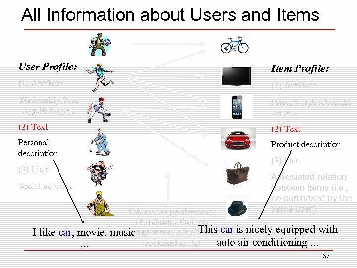 All Information about Users and Items User Profile: Item Profile: (1) Attribute Nationality, Sex, Age, Hobby, etc Price, Weight, Color, Br and, etc (2) Text Personal description Product description (3) link (3) Link Social network Observed preferences I like car, movie, … Associated relation between items (i. e. , co-purchased by the same user) (Purchases, Ratings, This page music views, play lists, car is nicely equipped with auto air conditioning … bookmarks, etc) 67
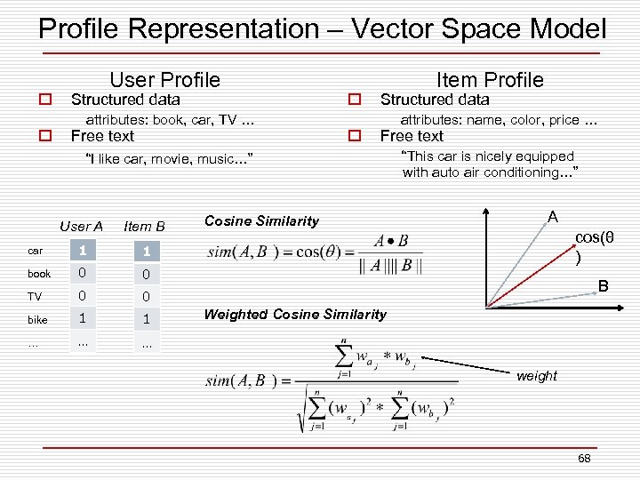 Profile Representation – Vector Space Model o o User Profile Structured data attributes: book, car, TV … Free text o o Item Profile Structured data attributes: name, color, price … Free text “I like car, movie, music…” User A Item B car 1 0 0 TV 0 0 bike 1 1 … … A 1 book Cosine Similarity “This car is nicely equipped with auto air conditioning…” … cos(θ ) B Weighted Cosine Similarity weight 68
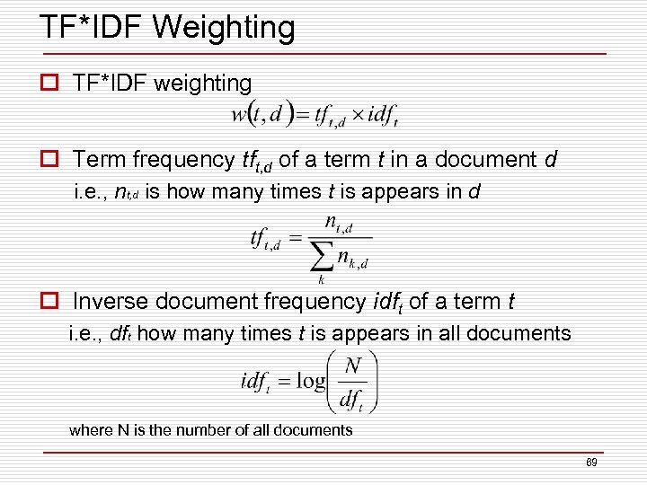 TF*IDF Weighting o TF*IDF weighting o Term frequency tft, d of a term t in a document d i. e. , nt, d is how many times t is appears in d o Inverse document frequency idft of a term t i. e. , dft how many times t is appears in all documents where N is the number of all documents 69
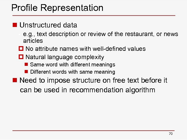 Profile Representation n Unstructured data • e. g. , text description or review of the restaurant, or news articles p No attribute names with well-defined values p Natural language complexity n Same word with different meanings n Different words with same meaning n Need to impose structure on free text before it can be used in recommendation algorithm 70
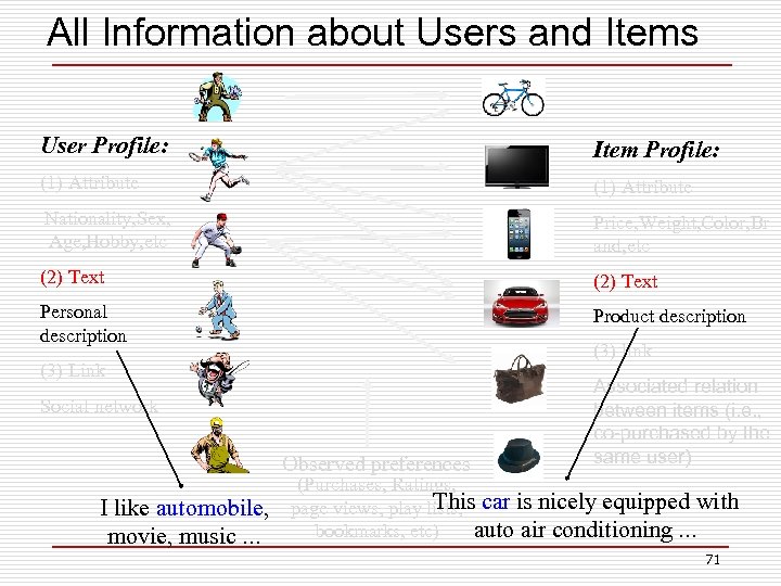 All Information about Users and Items User Profile: Item Profile: (1) Attribute Nationality, Sex, Age, Hobby, etc Price, Weight, Color, Br and, etc (2) Text Personal description Product description (3) link (3) Link Social network Observed preferences I like automobile, movie, music … Associated relation between items (i. e. , co-purchased by the same user) (Purchases, Ratings, This page views, play lists, car is nicely equipped with auto air conditioning … bookmarks, etc) 71
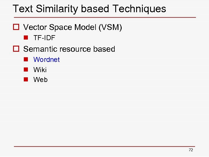 Text Similarity based Techniques o Vector Space Model (VSM) n TF-IDF o Semantic resource based n Wordnet n Wiki n Web 72
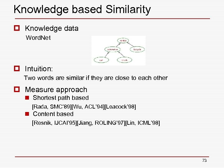 Knowledge based Similarity p Knowledge data Word. Net p Intuition: Two words are similar if they are close to each other p Measure approach n Shortest path based [Rada, SMC’ 89][Wu, ACL’ 94][Leacock’ 98] n Content based [Resnik, IJCAI’ 95][Jiang, ROLING’ 97][Lin, ICML’ 98] 73
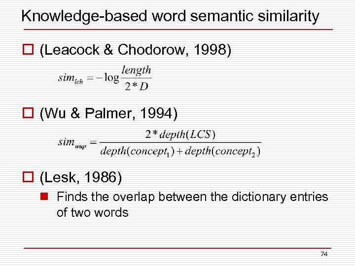 Knowledge-based word semantic similarity o (Leacock & Chodorow, 1998) o (Wu & Palmer, 1994) o (Lesk, 1986) n Finds the overlap between the dictionary entries of two words 74
 Text Similarity based Techniques o Vector Space Model (VSM) n TF-IDF o Semantic resource based n Wordnet n Wiki n Web 75
![Explicit Semantic Similarity (ESA) o Proposed by Gabrilovich [IJCAI’ 07] o Map text to Explicit Semantic Similarity (ESA) o Proposed by Gabrilovich [IJCAI’ 07] o Map text to](https://present5.com/presentation/8a42e9f8878d5abeef0048c800fed603/image-76.jpg) Explicit Semantic Similarity (ESA) o Proposed by Gabrilovich [IJCAI’ 07] o Map text to concepts (i. e. , vector) in Wiki o Calculate ESA score by common vector based measure (i. e. , cosine) 76
Explicit Semantic Similarity (ESA) o Proposed by Gabrilovich [IJCAI’ 07] o Map text to concepts (i. e. , vector) in Wiki o Calculate ESA score by common vector based measure (i. e. , cosine) 76
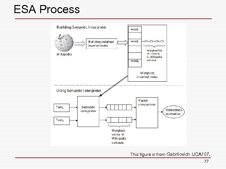 ESA Process This figure is from Gabrilovich IJCAI’ 07. 77
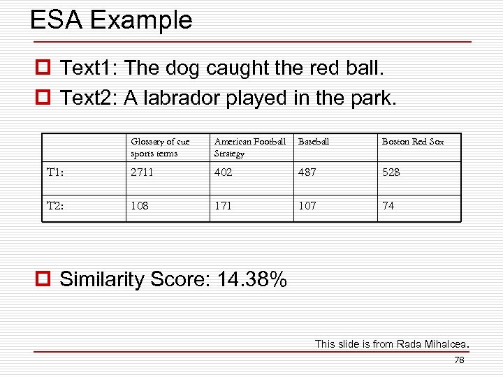 ESA Example p Text 1: The dog caught the red ball. p Text 2: A labrador played in the park. Glossary of cue sports terms American Football Strategy Baseball Boston Red Sox T 1: 2711 402 487 528 T 2: 108 171 107 74 p Similarity Score: 14. 38% This slide is from Rada Mihalcea. 78
 Text Similarity based Techniques o Vector Space Model (VSM) n TF-IDF o Semantic resource based n Wordnet n Wiki n Web 79
 Corpus based similarity o Corpus data n Web (search engine) o Intuition: n Two words are similar if they frequently occur in the same page n PMI-IR [Turney, ECML’ 01] 80
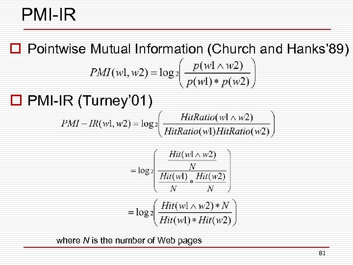 PMI-IR o Pointwise Mutual Information (Church and Hanks’ 89) o PMI-IR (Turney’ 01) where N is the number of Web pages 81
 Recommendation Approaches o Collaborative filtering o Content based strategies n n Association Rule Mining Text similarity based Clustering Classification o Hybrid approaches 82
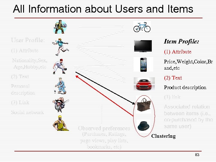 All Information about Users and Items User Profile: Item Profile: (1) Attribute Nationality, Sex, Age, Hobby, etc Price, Weight, Color, Br and, etc (2) Text Personal description Product description (3) link (3) Link Social network Observed preferences (Purchases, Ratings, page views, play lists, bookmarks, etc) Associated relation between items (i. e. , co-purchased by the same user) Clustering 83
 Clustering o K-means o Hierarchical Clustering 84
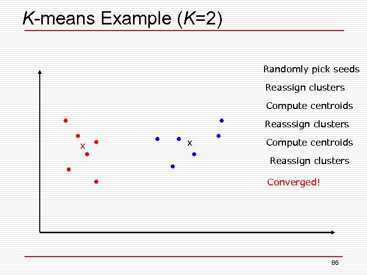
 K-means o Introduced by Mac. Queen, J. B. (1967) o Works when we know k, the number of clusters we want to find o Idea: n Randomly pick k points as the “centroids” of the k clusters n Loop: o For each point, put the point in the cluster to whose centroid it is closest o Recompute the cluster centroids o Repeat loop (until there is no change in clusters between two consecutive iterations. ) Iterative improvement of the objective function: Sum of the squared distance from each point to the centroid of its cluster 85
 K-means Example (K=2) Randomly pick seeds Reassign clusters Compute centroids Reasssign clusters x x Compute centroids Reassign clusters Converged! 86
 Clustering o K-means o Hierarchical Clustering 87
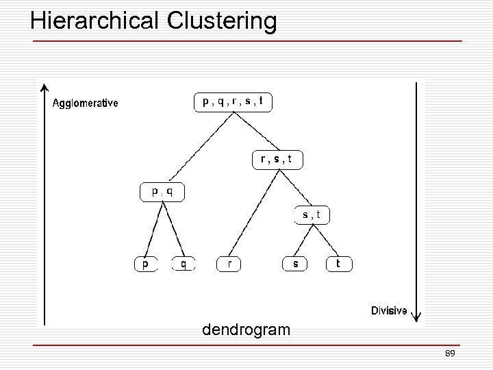
 Hierarchical Clustering o Two types: n Agglomerative (bottom up) n Divisive (top down) o Agglomerative: two groups are merged if distance between them is less than a threshold o Divisive: one group is split into two if intergroup distance more than a threshold o Can be expressed by an excellent graphical representation called dendrogram 88
 Hierarchical Clustering dendrogram 89
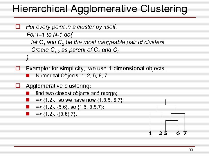 Hierarchical Agglomerative Clustering o Put every point in a cluster by itself. For I=1 to N-1 do{ let C 1 and C 2 be the most mergeable pair of clusters Create C 1, 2 as parent of C 1 and C 2 } o Example: for simplicity, we use 1 -dimensional objects. n Numerical Objects: 1, 2, 5, 6, 7 o Agglomerative clustering: n n find two closest objects and merge; => {1, 2}, so we have now {1. 5, 5, 6, 7}; => {1, 2}, {5, 6}, so {1. 5, 5. 5, 7}; => {1, 2}, {{5, 6}, 7}. 1 25 6 7 90
 Recommendation Approaches o Collaborative filtering o Content based strategies n n Association Rule Mining Text similarity based Clustering Classification o Hybrid approaches 91
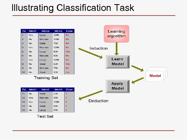 Illustrating Classification Task
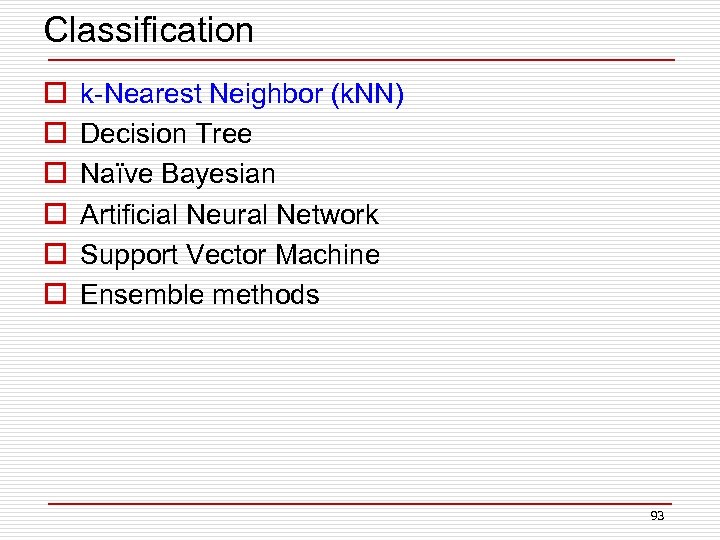 Classification o o o k-Nearest Neighbor (k. NN) Decision Tree Naïve Bayesian Artificial Neural Network Support Vector Machine Ensemble methods 93
 k-Nearest Neighbor Classification (k. NN) o k. NN does not build model from the training data. o Approach n To classify a test instance d, define k-neighborhood P as k nearest neighbors of d n Count number n of training instances in P that belong to class cj n Estimate Pr(cj|d) as n/k (majority vote) o No training is needed. Classification time is linear in training set size for each test case. o k is usually chosen empirically via a validation set or cross-validation by trying a range of k values. o Distance function is crucial, but depends on applications. 94
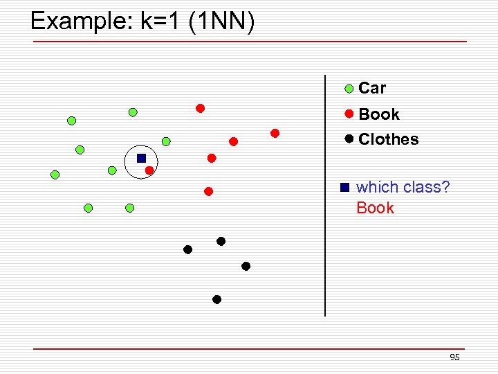 Example: k=1 (1 NN) Car Book Clothes which class? Book 95
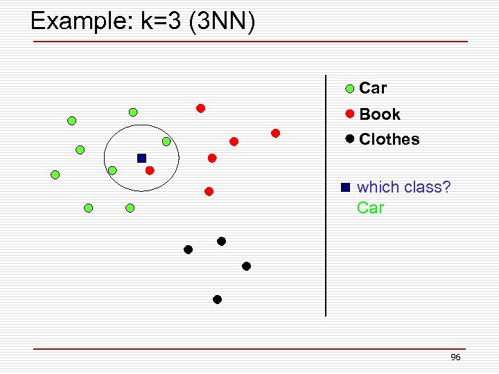 Example: k=3 (3 NN) Car Book Clothes which class? Car 96
 Discussion n Advantage o Nonparametric architecture o Simple o Powerful o Requires no training time n Disadvantage o Memory intensive o Classification/estimation is slow o Sensitive to k 97
 Classification o o o k-Nearest Neighbor (k. NN) Decision Tree Naïve Bayesian Artificial Neural Network Support Vector Machine Ensemble methods 98
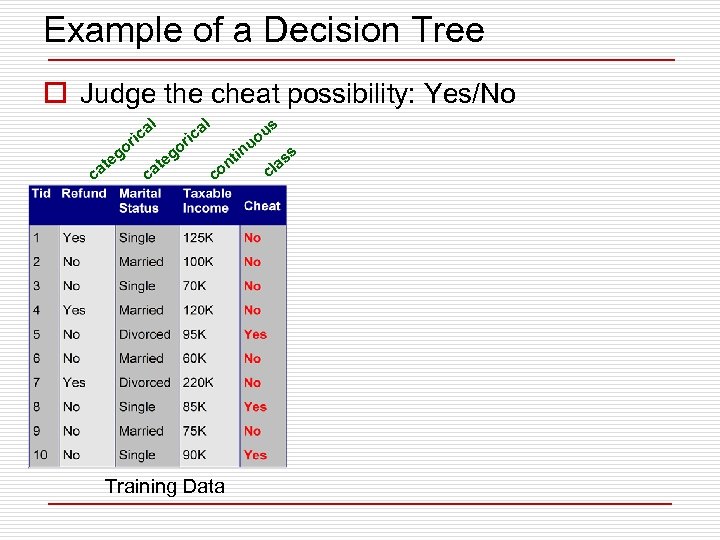 Example of a Decision Tree o Judge the cheat possibility: Yes/No al al ric o g te ca o ca g te s ric in t on c Training Data u uo c s as l
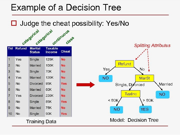 Example of a Decision Tree o Judge the cheat possibility: Yes/No al al ric o g te ca o ca g te s ric in t on c u uo s as l c Splitting Attributes Refund Yes No NO Mar. St Single, Divorced Tax. Inc < 80 K NO Training Data Married NO > 80 K YES Model: Decision Tree
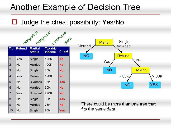 Another Example of Decision Tree o Judge the cheat possibility: Yes/No l ica or ca g te o g te ca l ica r in s ou u c t on s s la c Married Mar. St NO Single, Divorced Refund No Yes NO Tax. Inc < 80 K NO > 80 K YES There could be more than one tree that fits the same data!
 Decision Tree - Construction o Creating Decision Trees n Manual - Based on expert knowledge n Automated - Based on training data (DM) o Two main issues: n Issue #1: Which attribute to take for a split? n Issue #2: When to stop splitting?
 Classification o k-Nearest Neighbor (k. NN) o Decision Tree n CART n C 4. 5 o o Naïve Bayesian Artificial Neural Network Support Vector Machine Ensemble methods 103
 The CART Algorithm o Classification And Regression Trees o Developed by Breiman et al. in early 80’s. n Introduced tree-based modeling into the statistical mainstream n Rigorous approach involving cross-validation to select the optimal tree 104
 Key Idea Recursive Partitioning o Take all of your data. o Consider all possible values of all variables. o Select the variable/value (X=t 1) that produces the greatest “separation” in the target. o (X=t 1) is called a “split”. o If X< t 1 then send the data to the “left”; otherwise, send data point to the “right”. o Now repeat same process on these two “nodes” o You get a “tree” o Note: CART only uses binary splits. 105
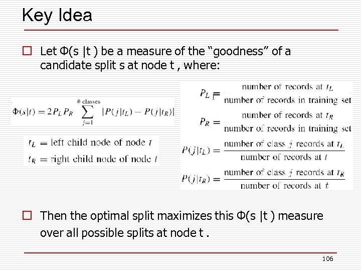 Key Idea o Let Φ(s |t ) be a measure of the “goodness” of a candidate split s at node t , where: o Then the optimal split maximizes this Φ(s |t ) measure over all possible splits at node t. 106
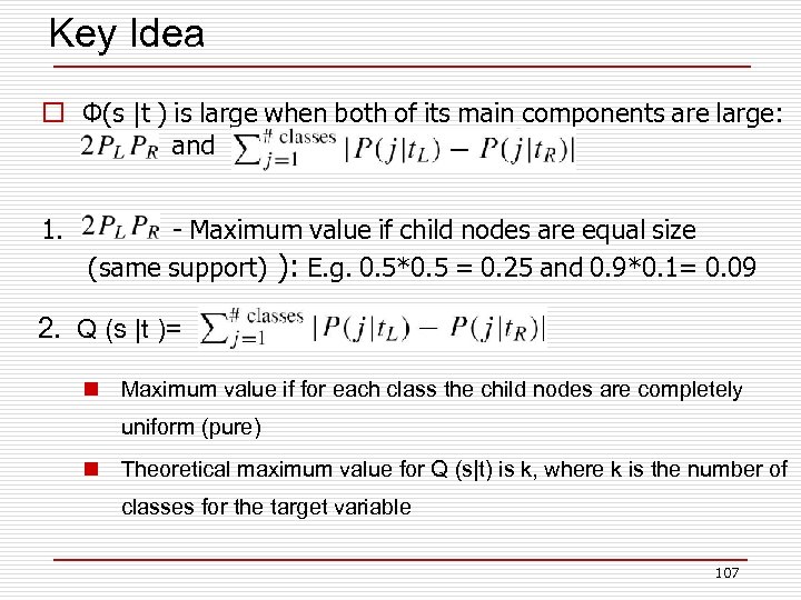 Key Idea o Φ(s |t ) is large when both of its main components are large: and 1. - Maximum value if child nodes are equal size (same support) ): E. g. 0. 5*0. 5 = 0. 25 and 0. 9*0. 1= 0. 09 2. Q (s |t )= n Maximum value if for each class the child nodes are completely uniform (pure) n Theoretical maximum value for Q (s|t) is k, where k is the number of classes for the target variable 107
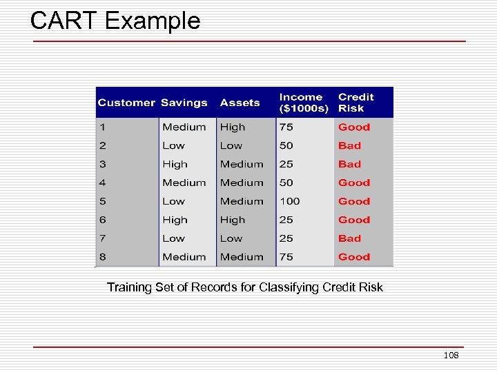 CART Example Training Set of Records for Classifying Credit Risk 108
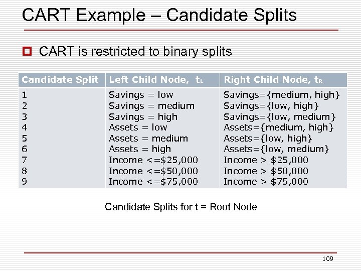 CART Example – Candidate Splits p CART is restricted to binary splits Candidate Split Left Child Node, t. L Right Child Node, t. R 1 2 3 4 5 6 7 8 9 Savings = low Savings = medium Savings = high Assets = low Assets = medium Assets = high Income <=$25, 000 Income <=$50, 000 Income <=$75, 000 Savings={medium, high} Savings={low, medium} Assets={medium, high} Assets={low, medium} Income > $25, 000 Income > $50, 000 Income > $75, 000 Candidate Splits for t = Root Node 109
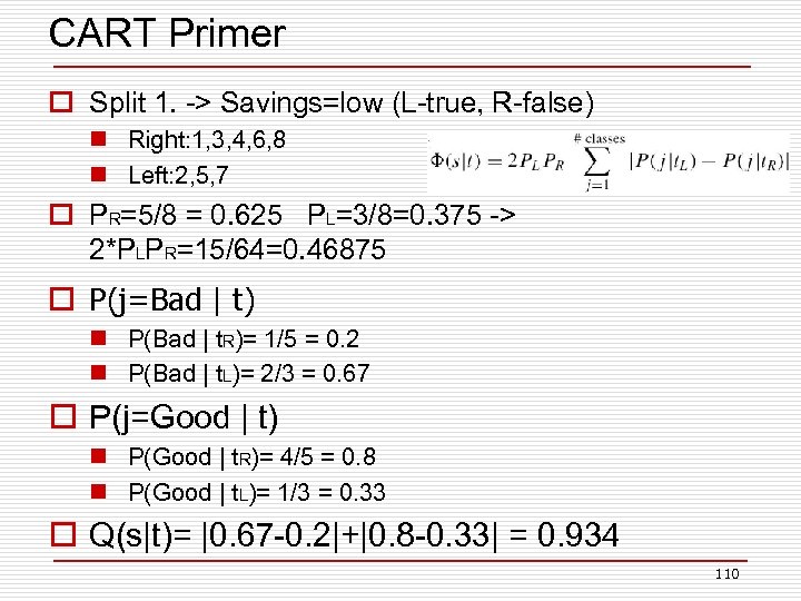 CART Primer o Split 1. -> Savings=low (L-true, R-false) n Right: 1, 3, 4, 6, 8 n Left: 2, 5, 7 o PR=5/8 = 0. 625 PL=3/8=0. 375 -> 2*PLPR=15/64=0. 46875 o P(j=Bad | t) n P(Bad | t. R)= 1/5 = 0. 2 n P(Bad | t. L)= 2/3 = 0. 67 o P(j=Good | t) n P(Good | t. R)= 4/5 = 0. 8 n P(Good | t. L)= 1/3 = 0. 33 o Q(s|t)= |0. 67 -0. 2|+|0. 8 -0. 33| = 0. 934 110
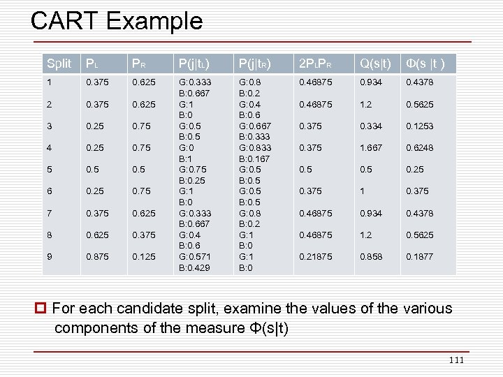 CART Example Split PL PR P(j|t. L) P(j|t. R) 2 PLPR Q(s|t) Φ(s |t ) 1 0. 375 0. 625 0. 934 0. 4378 0. 375 0. 625 0. 46875 1. 2 0. 5625 3 0. 25 0. 75 0. 334 0. 1253 4 0. 25 0. 75 0. 375 1. 667 0. 6248 5 0. 25 6 0. 25 0. 75 0. 375 1 0. 375 7 0. 375 0. 625 0. 46875 0. 934 0. 4378 8 0. 625 0. 375 0. 46875 1. 2 0. 5625 9 0. 875 0. 125 G: 0. 8 B: 0. 2 G: 0. 4 B: 0. 6 G: 0. 667 B: 0. 333 G: 0. 833 B: 0. 167 G: 0. 5 B: 0. 5 G: 0. 8 B: 0. 2 G: 1 B: 0 0. 46875 2 G: 0. 333 B: 0. 667 G: 1 B: 0 G: 0. 5 B: 0. 5 G: 0 B: 1 G: 0. 75 B: 0. 25 G: 1 B: 0 G: 0. 333 B: 0. 667 G: 0. 4 B: 0. 6 G: 0. 571 B: 0. 429 0. 21875 0. 858 0. 1877 p For each candidate split, examine the values of the various components of the measure Φ(s|t) 111
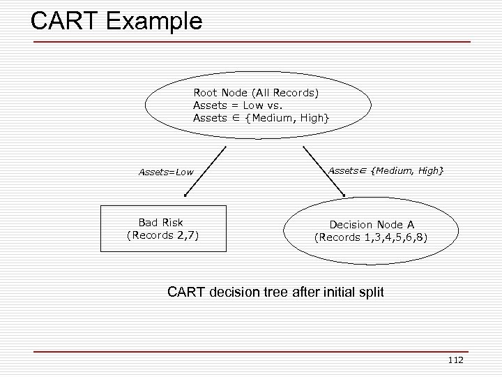 CART Example Root Node (All Records) Assets = Low vs. Assets ∈ {Medium, High} Assets=Low Bad Risk (Records 2, 7) Assets∈ {Medium, High} Decision Node A (Records 1, 3, 4, 5, 6, 8) CART decision tree after initial split 112
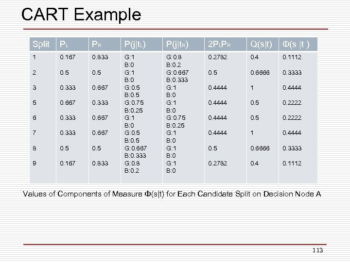 CART Example Split PL PR P(j|t. L) P(j|t. R) 2 PLPR Q(s|t) Φ(s |t ) 1 0. 167 0. 833 0. 4 0. 1112 0. 5 0. 6666 0. 3333 3 0. 333 0. 667 0. 4444 1 0. 4444 5 0. 667 0. 333 0. 4444 0. 5 0. 2222 6 0. 333 0. 667 0. 4444 0. 5 0. 2222 7 0. 333 0. 667 0. 4444 1 0. 4444 8 0. 5 0. 6666 0. 3333 9 0. 167 0. 833 G: 0. 8 B: 0. 2 G: 0. 667 B: 0. 333 G: 1 B: 0 G: 0. 75 B: 0. 25 G: 1 B: 0 0. 2782 2 G: 1 B: 0 G: 0. 5 B: 0. 5 G: 0. 75 B: 0. 25 G: 1 B: 0 G: 0. 5 B: 0. 5 G: 0. 667 B: 0. 333 G: 0. 8 B: 0. 2782 0. 4 0. 1112 Values of Components of Measure Φ(s|t) for Each Candidate Split on Decision Node A 113
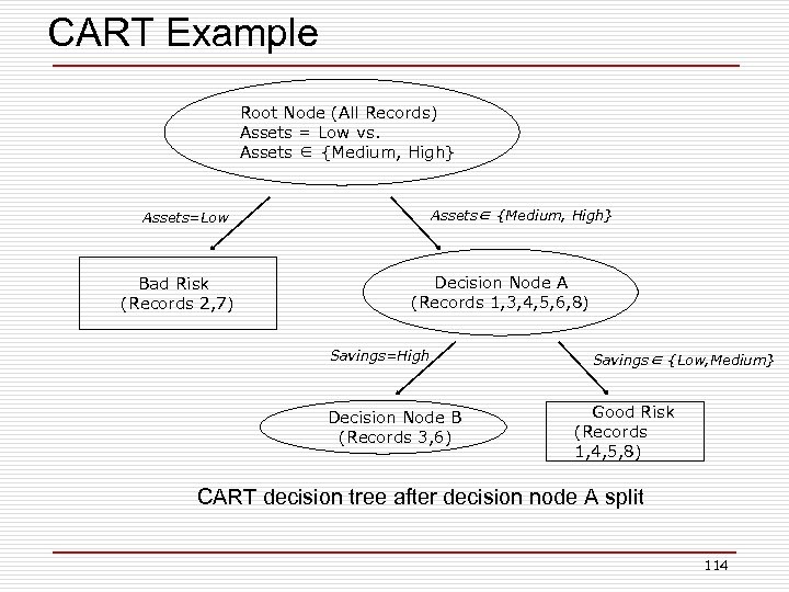 CART Example Root Node (All Records) Assets = Low vs. Assets ∈ {Medium, High} Assets=Low Bad Risk (Records 2, 7) Decision Node A (Records 1, 3, 4, 5, 6, 8) Savings=High Decision Node B (Records 3, 6) Savings∈ {Low, Medium} Good Risk (Records 1, 4, 5, 8) CART decision tree after decision node A split 114
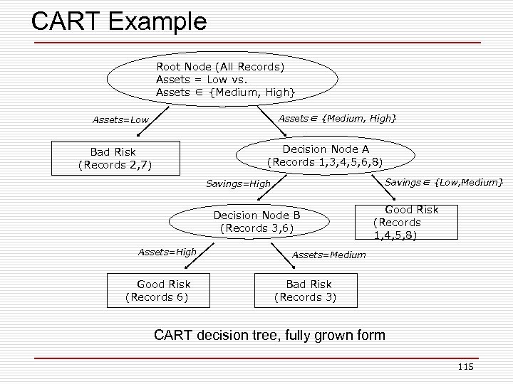 CART Example Root Node (All Records) Assets = Low vs. Assets ∈ {Medium, High} Assets=Low Decision Node A (Records 1, 3, 4, 5, 6, 8) Bad Risk (Records 2, 7) Savings∈ {Low, Medium} Savings=High Decision Node B (Records 3, 6) Assets=High Good Risk (Records 6) Good Risk (Records 1, 4, 5, 8) Assets=Medium Bad Risk (Records 3) CART decision tree, fully grown form 115
 Classification o k-Nearest Neighbor (k. NN) o Decision Tree n CART n C 4. 5 o o Naïve Bayesian Artificial Neural Network Support Vector Machine Ensemble methods 116
 The C 4. 5 Algorithm o Proposed by Quinlan in 1993 o An internal node represents a test on an attribute. o A branch represents an outcome of the test, e. g. , Color=red. o A leaf node represents a class label or class label distribution. o At each node, one attribute is chosen to split training examples into distinct classes as much as possible o A new case is classified by following a matching path to a leaf node. 117
 The C 4. 5 Algorithm o Differences between CART and C 4. 5: n Unlike CART, the C 4. 5 algorithm is not restricted to binary splits. o It produces a separate branch for each value of the categorical attribute. n C 4. 5 method for measuring node homogeneity is different from the CART. 118
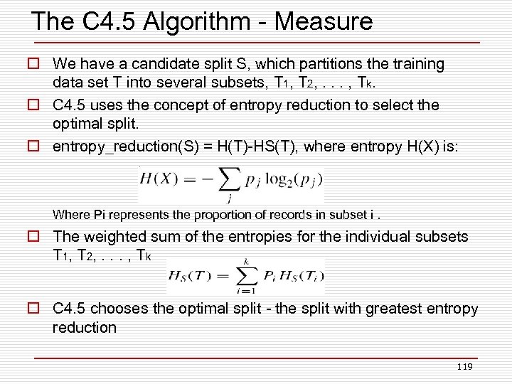 The C 4. 5 Algorithm - Measure o We have a candidate split S, which partitions the training data set T into several subsets, T 1, T 2, . . . , Tk. o C 4. 5 uses the concept of entropy reduction to select the optimal split. o entropy_reduction(S) = H(T)-HS(T), where entropy H(X) is: Where Pi represents the proportion of records in subset i. o The weighted sum of the entropies for the individual subsets T 1, T 2, . . . , T k o C 4. 5 chooses the optimal split - the split with greatest entropy reduction 119
 Classification o o o k-Nearest Neighbor (k. NN) Decision Tree Naïve Bayesian Artificial Neural Network Support Vector Machine Ensemble methods 120
 Bayes Rule o Recommender system question n Li is the class for item i (i. e. , that the user likes item i) n A is the set of features associated with item i o Estimate p(Li|A) o p(Li |A) = p(A| Li) p(Li) / p(A) o We can always restate a conditional probability in terms of n The reverse condition p(A| Li) n Two prior probabilities o p(Li) o p(A) o Often the reverse condition is easier to know n We can count how often a feature appears in items the user liked n Frequentist assumption 121
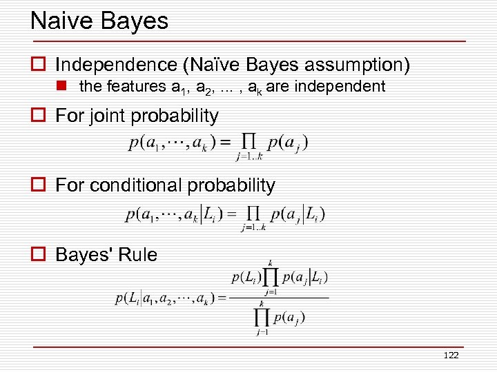 Naive Bayes o Independence (Naïve Bayes assumption) n the features a 1, a 2, . . . , ak are independent o For joint probability o For conditional probability o Bayes' Rule 122
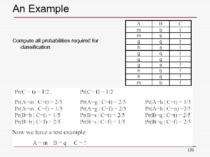 An Example Compute all probabilities required for classification 123
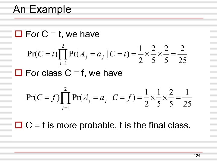 An Example o For C = t, we have o For class C = f, we have o C = t is more probable. t is the final class. 124
 Naïve Bayesian Classifier o Advantages: n Easy to implement n Very efficient n Good results obtained in many applications o Disadvantages n Assumption: class conditional independence, therefore loss of accuracy when the assumption is seriously violated (those highly correlated data sets) 125
 Classification o o o K-Nearest Neighbor (k. NN) Decision Tree Naïve Bayesian Artificial Neural Network Support Vector Machine Ensemble methods 126
 References for Machine Learning o T. Mitchell, Machine Learning, Mc. Graw Hill, 1997 o C. M. Bishop, Pattern Recognition and Machine Learning, Springer, 2006 o T. Hastie, R. Tibshirani and J. Friedman, The Elements of Statistical Learning, Springer, 2001. o V. Vapnik, Statistical Learning Theory, Wiley-Interscience, 1998. o Y. Kodratoff, R. S. Michalski, Machine Learning: An Artificial Intelligence Approach, Volume III, Morgan Kaufmann, 1990 127
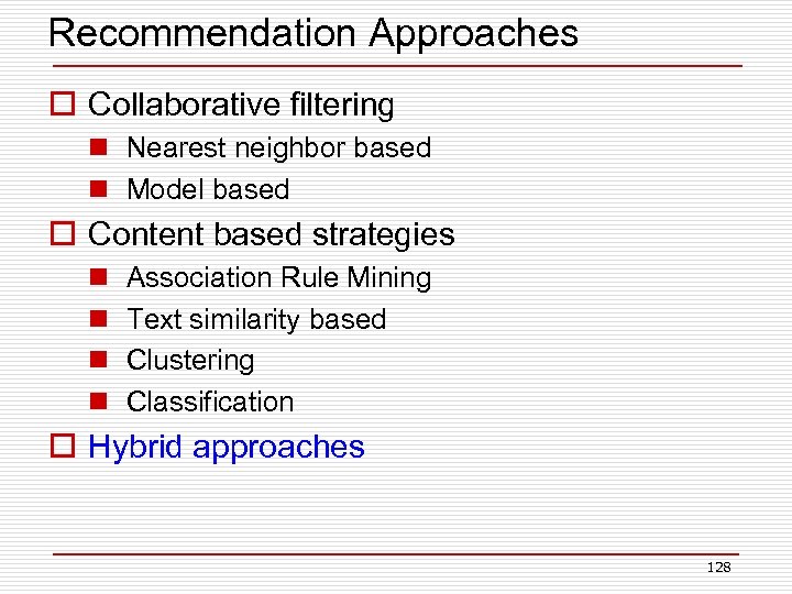 Recommendation Approaches o Collaborative filtering n Nearest neighbor based n Model based o Content based strategies n n Association Rule Mining Text similarity based Clustering Classification o Hybrid approaches 128
 The Netflix Prize Slides here are from Yehuda Koren.
 Netflix o Movie rentals by DVD (mail) and online (streaming) o 100 k movies, 10 million customers o Ships 1. 9 million disks to customers each day n 50 warehouses in the US n Complex logistics problem o Employees: 2000 n But relatively few in engineering/software n And only a few people working on recommender systems o Moving towards online delivery of content o Significant interaction of customers with Web site 130
 The $1 Million Question 131
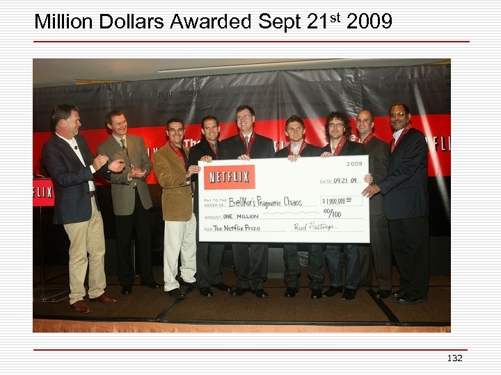 Million Dollars Awarded Sept 21 st 2009 132
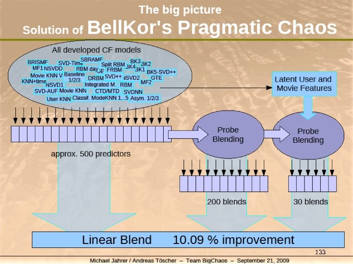 133
133
 Lessons Learned o Scale is important n e. g. , stochastic gradient descent on sparse matrices o Latent factor models work well on this problem n Previously had not been explored for recommender systems o Understanding your data is important, e. g. , timeeffects o Combining models works surprisingly well n But final 10% improvement can probably be achieved by judiciously combining about 10 models rather than 1000’s n This is likely what Netflix will do in practice 134
 Useful References o Y. Koren, Collaborative filtering with temporal dynamics, ACM SIGKDD Conference 2009 o Y. Koren, R. Bell, C. Volinsky, Matrix factorization techniques for recommender systems, IEEE Computer, 2009 o Y. Koren, Factor in the neighbors: scalable and accurate collaborative filtering, ACM Transactions on Knowledge Discovery in Data, 2010 135
 Thank you! 136


