a1ffdf92f322d4a3495126c35a1c384d.ppt
- Количество слайдов: 85
 Data Mining Algorithms Classification
 Classification Outline Goal: Provide an overview of the classification problem and introduce some of the basic algorithms Classification Problem Overview Classification Techniques – Regression – Distance – Decision Trees – Rules – Neural Networks
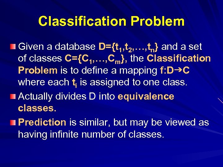 Classification Problem Given a database D={t 1, t 2, …, tn} and a set of classes C={C 1, …, Cm}, the Classification Problem is to define a mapping f: Dg. C where each ti is assigned to one class. Actually divides D into equivalence classes. Prediction is similar, but may be viewed as having infinite number of classes.
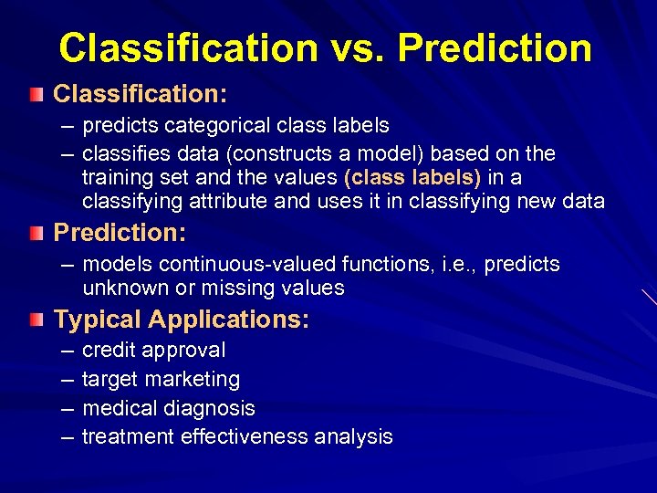 Classification vs. Prediction Classification: – predicts categorical class labels – classifies data (constructs a model) based on the training set and the values (class labels) in a classifying attribute and uses it in classifying new data Prediction: – models continuous-valued functions, i. e. , predicts unknown or missing values Typical Applications: – – credit approval target marketing medical diagnosis treatment effectiveness analysis
 Classification Examples Teachers classify students’ grades as A, B, C, D, or F. Predict when a disaster will strike Identify individuals with credit risks. Speech recognition Pattern recognition
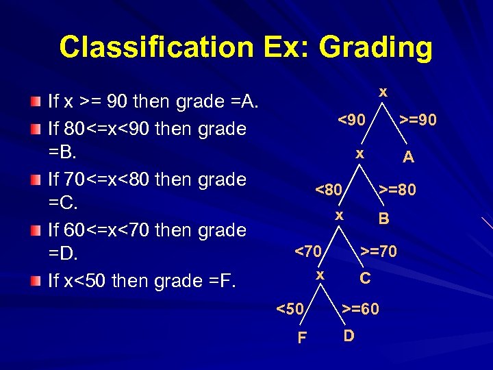 Classification Ex: Grading If x >= 90 then grade =A. If 80<=x<90 then grade =B. If 70<=x<80 then grade =C. If 60<=x<70 then grade =D. If x<50 then grade =F. x <90 >=90 x <80 x <70 x <50 F A >=80 B >=70 C >=60 D
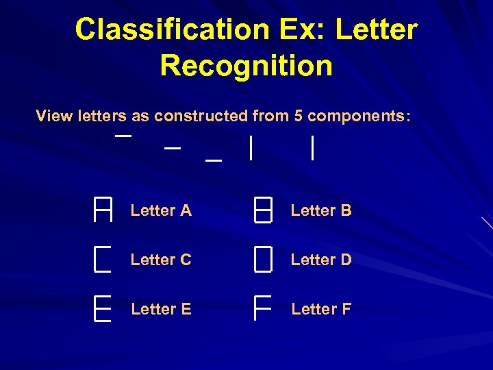 Classification Ex: Letter Recognition View letters as constructed from 5 components: Letter A Letter B Letter C Letter D Letter E Letter F
 Classification Techniques Approach: 1. Create specific model by evaluating training data (or using domain experts’ knowledge). 2. Apply model developed to new data. Classes must be predefined Most common techniques use Decision Trees, Neural Networks, or are based on distances or statistical methods.
 Classification—A 2 Step Process Model construction: describing a set of predetermined classes – Each tuple/sample is assumed to belong to a predefined class, as determined by the class label attribute – The set of tuples used for model construction: training set – The model is represented as classification rules, decision trees, or mathematical formulae
 Classification—A 2 Step Process Model usage: for classifying future or unknown objects – Estimate accuracy of the model The known label of test sample is compared with the classified result from the model Accuracy rate is the percentage of test set samples that are correctly classified by the model Test set is independent of training set, otherwise over-fitting will occur
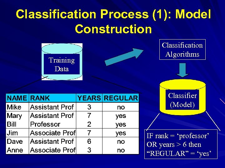 Classification Process (1): Model Construction Training Data Classification Algorithms Classifier (Model) IF rank = ‘professor’ OR years > 6 then “REGULAR” = ‘yes’
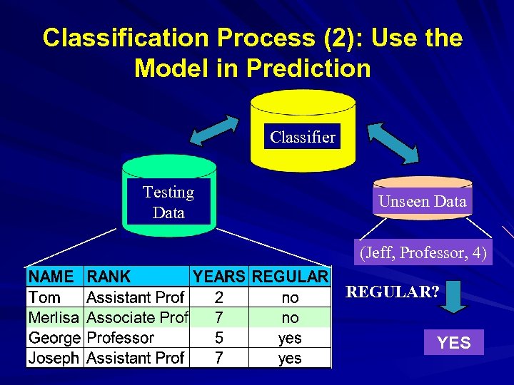 Classification Process (2): Use the Model in Prediction Classifier Testing Data Unseen Data (Jeff, Professor, 4) REGULAR? YES
 Supervised vs. Unsupervised Learning Supervised learning (classification) – Supervision: The training data (observations, measurements, etc. ) are accompanied by labels indicating the class of the observations – New data is classified based on the training set Unsupervised learning (clustering) – The class labels of training data is unknown – Given a set of measurements, observations, etc. with the aim of establishing the existence of classes or clusters in the data
 Issues in Classification Missing Data – Ignore – Replace with assumed value Measuring Performance – Classification accuracy on test data – Confusion matrix – OC Curve
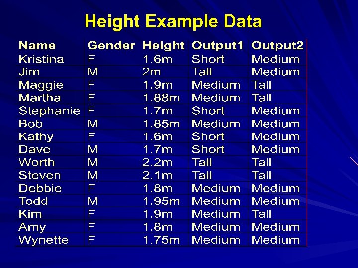 Height Example Data
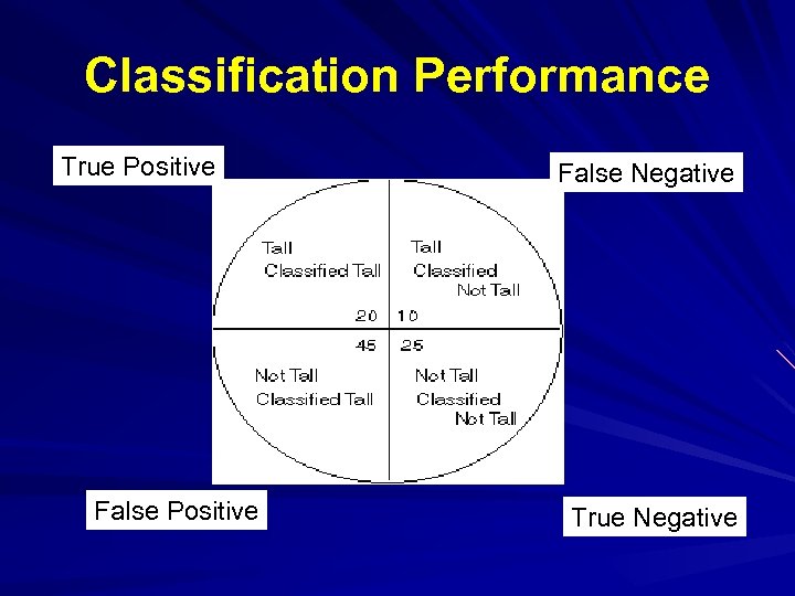 Classification Performance True Positive False Negative True Negative
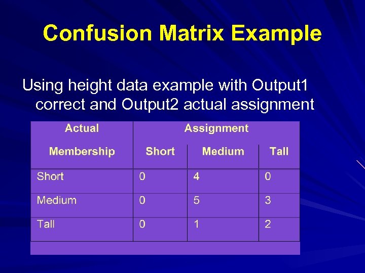 Confusion Matrix Example Using height data example with Output 1 correct and Output 2 actual assignment
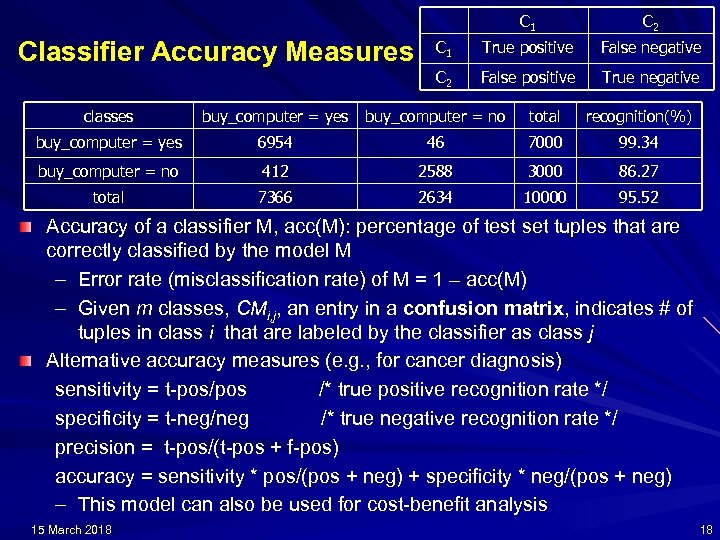 C 1 Classifier Accuracy Measures C 2 C 1 True positive False negative C 2 False positive True negative classes buy_computer = yes buy_computer = no total recognition(%) buy_computer = yes 6954 46 7000 99. 34 buy_computer = no 412 2588 3000 86. 27 total 7366 2634 10000 95. 52 Accuracy of a classifier M, acc(M): percentage of test set tuples that are correctly classified by the model M – Error rate (misclassification rate) of M = 1 – acc(M) – Given m classes, CMi, j, an entry in a confusion matrix, indicates # of tuples in class i that are labeled by the classifier as class j Alternative accuracy measures (e. g. , for cancer diagnosis) sensitivity = t-pos/pos /* true positive recognition rate */ specificity = t-neg/neg /* true negative recognition rate */ precision = t-pos/(t-pos + f-pos) accuracy = sensitivity * pos/(pos + neg) + specificity * neg/(pos + neg) – This model can also be used for cost-benefit analysis 15 March 2018 18
 Evaluating the Accuracy of a Classifier or Predictor (I) Holdout method – Given data is randomly partitioned into two independent sets Training set (e. g. , 2/3) for model construction Test set (e. g. , 1/3) for accuracy estimation – Random sampling: a variation of holdout Repeat holdout k times, accuracy = avg. of the accuracies obtained Cross-validation (k-fold, where k = 10 is most popular) – Randomly partition the data into k mutually exclusive subsets, each approximately equal size – At i-th iteration, use Di as test set and others as training set – Leave-one-out: k folds where k = # of tuples, for small sized data – Stratified cross-validation: folds are stratified so that class dist. in each fold is approx. the same as that in the initial data 15 March 2018 19
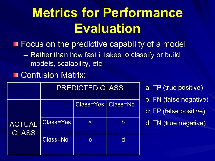 Metrics for Performance Evaluation Focus on the predictive capability of a model – Rather than how fast it takes to classify or build models, scalability, etc. Confusion Matrix: PREDICTED CLASS Class=Yes Class=No ACTUAL Class=Yes CLASS Class=No a b c d a: TP (true positive) b: FN (false negative) c: FP (false positive) d: TN (true negative)
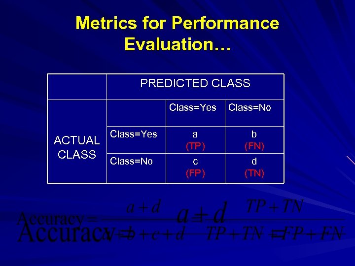 Metrics for Performance Evaluation… PREDICTED CLASS Class=Yes ACTUAL CLASS Class=No Class=Yes a (TP) b (FN) Class=No c (FP) d (TN)
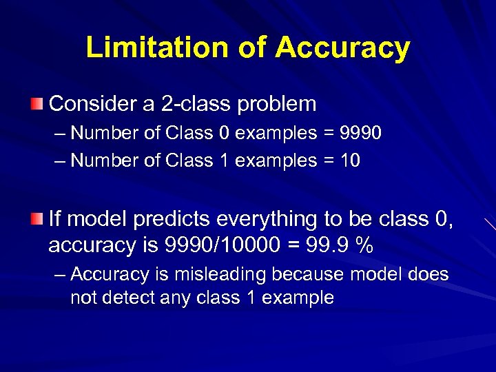 Limitation of Accuracy Consider a 2 -class problem – Number of Class 0 examples = 9990 – Number of Class 1 examples = 10 If model predicts everything to be class 0, accuracy is 9990/10000 = 99. 9 % – Accuracy is misleading because model does not detect any class 1 example
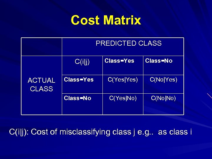 Cost Matrix PREDICTED CLASS C(i|j) Class=Yes Class=No Class=Yes C(Yes|Yes) C(No|Yes) Class=No ACTUAL CLASS C(Yes|No) C(No|No) C(i|j): Cost of misclassifying class j e. g. . as class i
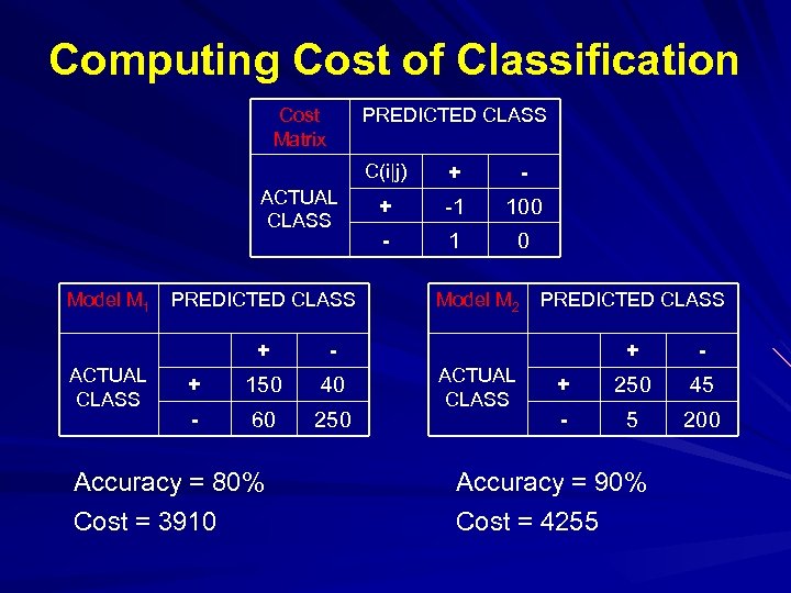 Computing Cost of Classification Cost Matrix PREDICTED CLASS C(i|j) ACTUAL CLASS Model M 1 PREDICTED CLASS + ACTUAL CLASS 150 40 - 60 250 - + -1 100 - 1 0 Model M 2 PREDICTED CLASS - + + Accuracy = 80% Cost = 3910 + ACTUAL CLASS - + 250 45 - 5 200 Accuracy = 90% Cost = 4255
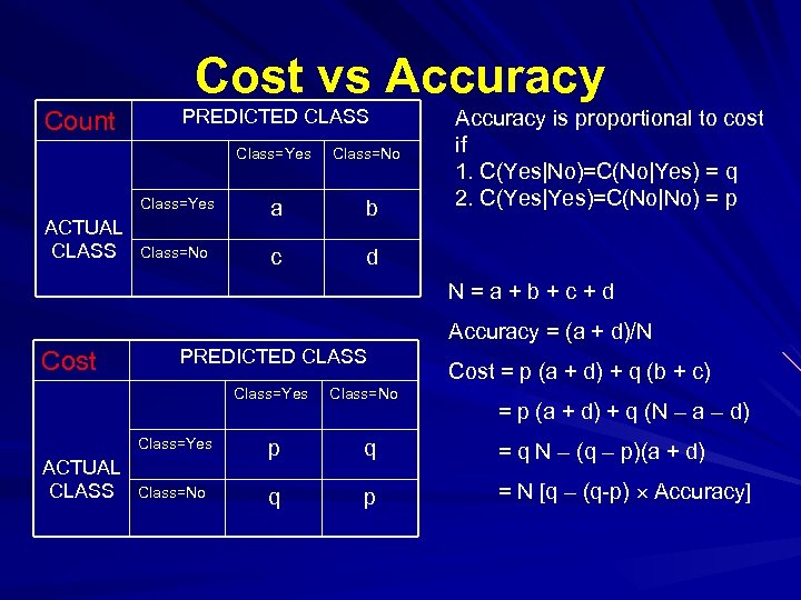 Cost vs Accuracy Count PREDICTED CLASS Class=Yes Class=No Class=Yes ACTUAL CLASS a b Class=No c Accuracy is proportional to cost if 1. C(Yes|No)=C(No|Yes) = q 2. C(Yes|Yes)=C(No|No) = p d N=a+b+c+d Accuracy = (a + d)/N Cost PREDICTED CLASS Class=Yes Class=No Cost = p (a + d) + q (b + c) = p (a + d) + q (N – a – d) Class=Yes ACTUAL CLASS p q = q N – (q – p)(a + d) Class=No q p = N [q – (q-p) Accuracy]
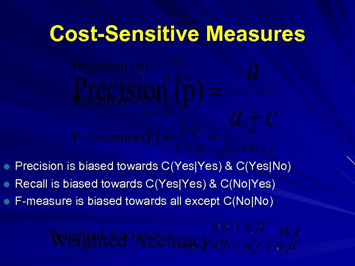 Cost-Sensitive Measures l l l Precision is biased towards C(Yes|Yes) & C(Yes|No) Recall is biased towards C(Yes|Yes) & C(No|Yes) F-measure is biased towards all except C(No|No)
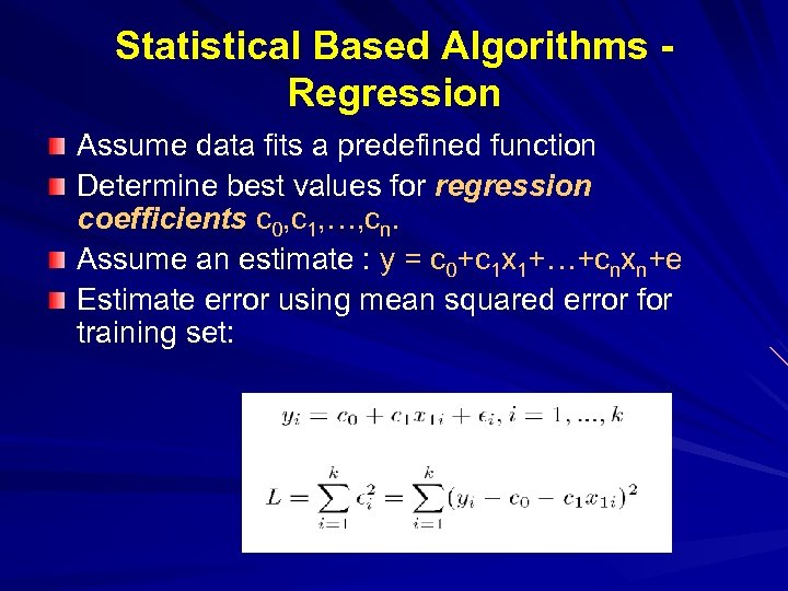 Statistical Based Algorithms Regression Assume data fits a predefined function Determine best values for regression coefficients c 0, c 1, …, cn. Assume an estimate : y = c 0+c 1 x 1+…+cnxn+e Estimate error using mean squared error for training set:
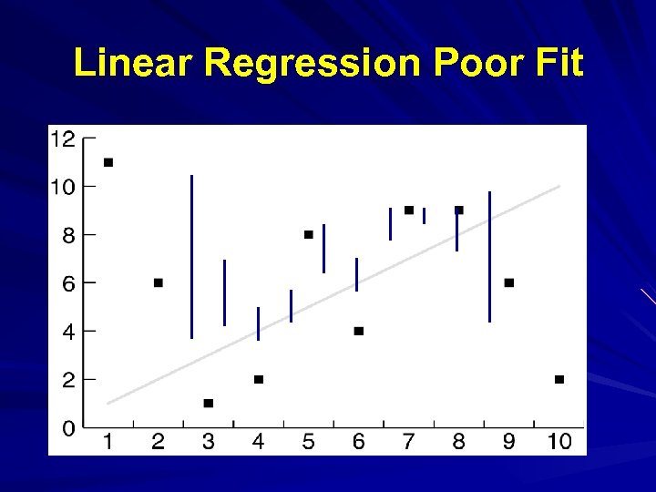 Linear Regression Poor Fit
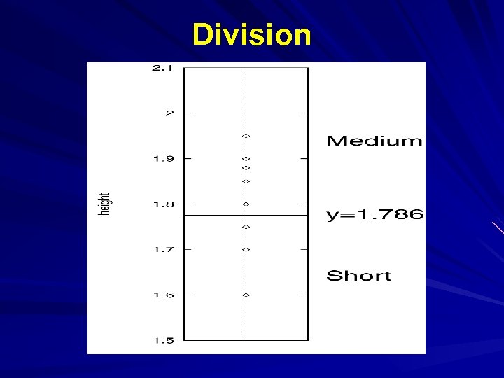
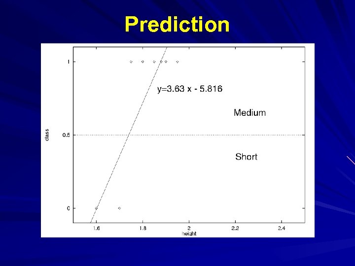
 Classification Using Regression Division: Use regression function to divide area into regions. Prediction: Use regression function to predict a class membership function. Input includes desired class.
 Division
 Prediction
 Bayesian Classification: Why? Probabilistic learning: Calculate explicit probabilities for hypothesis, among the most practical approaches to certain types of learning problems Incremental: Each training example can incrementally increase/decrease the probability that a hypothesis is correct. Prior knowledge can be combined with observed data. Probabilistic prediction: Predict multiple hypotheses, weighted by their probabilities Standard: Even when Bayesian methods are computationally intractable, they can provide a standard of optimal decision making against which other methods can be measured
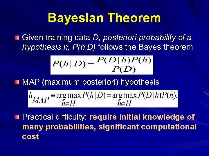 Bayesian Theorem Given training data D, posteriori probability of a hypothesis h, P(h|D) follows the Bayes theorem MAP (maximum posteriori) hypothesis Practical difficulty: require initial knowledge of many probabilities, significant computational cost
 Bayesian classification The classification problem may be formalized using a-posteriori probabilities: P(C|X) = prob. that the sample tuple X=
 Estimating a-posteriori probabilities Bayes theorem: P(C|X) = P(X|C)·P(C) / P(X) is constant for all classes P(C) = relative freq of class C samples C such that P(C|X) is maximum = C such that P(X|C)·P(C) is maximum Problem: computing P(X|C) is unfeasible!
 Naïve Bayesian Classification Naïve assumption: attribute independence P(x 1, …, xk|C) = P(x 1|C)·…·P(xk|C) If i-th attribute is categorical: P(xi|C) is estimated as the relative freq of samples having value xi as i-th attribute in class C If i-th attribute is continuous: P(xi|C) is estimated thru a Gaussian density function Computationally easy in both cases
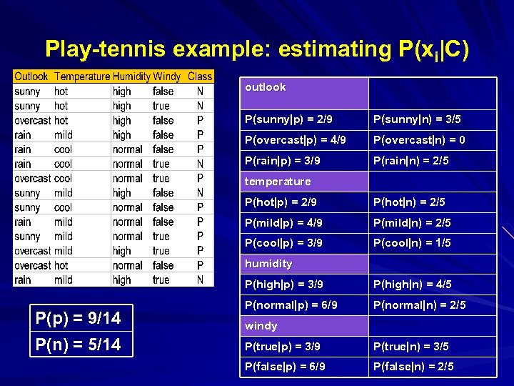 Play-tennis example: estimating P(xi|C) outlook P(sunny|p) = 2/9 P(sunny|n) = 3/5 P(overcast|p) = 4/9 P(overcast|n) = 0 P(rain|p) = 3/9 P(rain|n) = 2/5 temperature P(hot|p) = 2/9 P(hot|n) = 2/5 P(mild|p) = 4/9 P(mild|n) = 2/5 P(cool|p) = 3/9 P(cool|n) = 1/5 humidity P(high|p) = 3/9 P(p) = 9/14 P(n) = 5/14 P(high|n) = 4/5 P(normal|p) = 6/9 P(normal|n) = 2/5 windy P(true|p) = 3/9 P(true|n) = 3/5 P(false|p) = 6/9 P(false|n) = 2/5
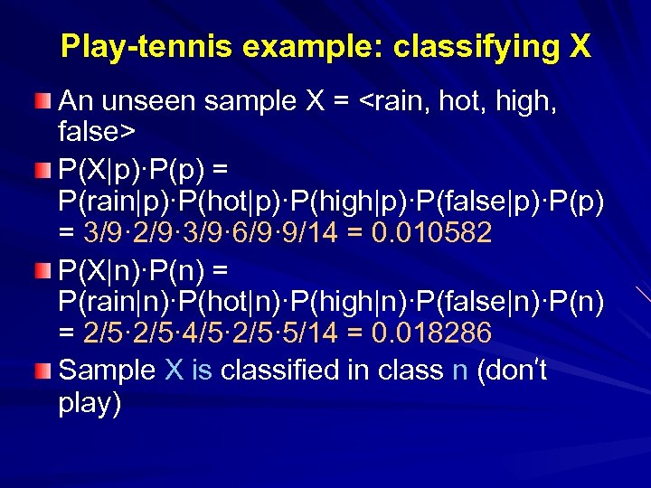 Play-tennis example: classifying X An unseen sample X =
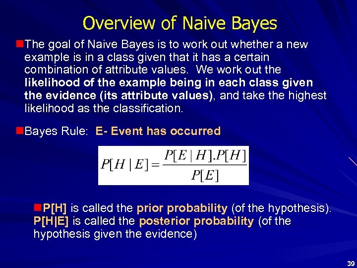 Overview of Naive Bayes n. The goal of Naive Bayes is to work out whether a new example is in a class given that it has a certain combination of attribute values. We work out the likelihood of the example being in each class given the evidence (its attribute values), and take the highest likelihood as the classification. n. Bayes Rule: E- Event has occurred n. P[H] is called the prior probability (of the hypothesis). P[H|E] is called the posterior probability (of the hypothesis given the evidence) 39
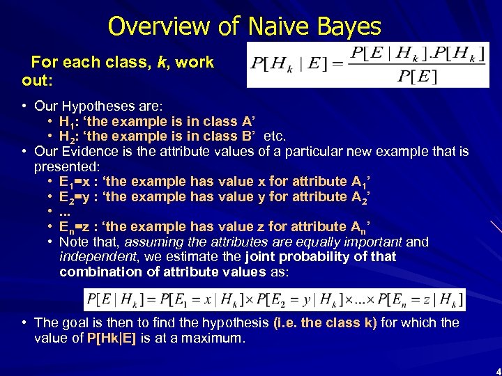 Overview of Naive Bayes For each class, k, work out: • Our Hypotheses are: • H 1: ‘the example is in class A’ • H 2: ‘the example is in class B’ etc. • Our Evidence is the attribute values of a particular new example that is presented: • E 1=x : ‘the example has value x for attribute A 1’ • E 2=y : ‘the example has value y for attribute A 2’ • . . . • En=z : ‘the example has value z for attribute An’ • Note that, assuming the attributes are equally important and independent, we estimate the joint probability of that combination of attribute values as: • The goal is then to find the hypothesis (i. e. the class k) for which the value of P[Hk|E] is at a maximum. 4
![Overview of Naive Bayes • For categorical variables we use simple proportions. P[Ei=x|Hk] = Overview of Naive Bayes • For categorical variables we use simple proportions. P[Ei=x|Hk] =](https://present5.com/presentation/a1ffdf92f322d4a3495126c35a1c384d/image-41.jpg) Overview of Naive Bayes • For categorical variables we use simple proportions. P[Ei=x|Hk] = no. of training egs in class k having value x for attribute A i number of training examples in class k • For continuous variables we assume a normal (Gaussian) distribution, and use the mean ( ) and standard deviation ( ) to compute the conditional probabilities. P[Ei =x |Hk] = 41
Overview of Naive Bayes • For categorical variables we use simple proportions. P[Ei=x|Hk] = no. of training egs in class k having value x for attribute A i number of training examples in class k • For continuous variables we assume a normal (Gaussian) distribution, and use the mean ( ) and standard deviation ( ) to compute the conditional probabilities. P[Ei =x |Hk] = 41
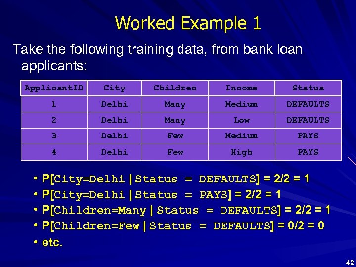 Worked Example 1 Take the following training data, from bank loan applicants: Applicant. ID City Children Income Status 1 Delhi Many Medium DEFAULTS 2 Delhi Many Low DEFAULTS 3 Delhi Few Medium PAYS 4 Delhi Few High PAYS • • • P[City=Delhi | Status = DEFAULTS] = 2/2 = 1 P[City=Delhi | Status = PAYS] = 2/2 = 1 P[Children=Many | Status = DEFAULTS] = 2/2 = 1 P[Children=Few | Status = DEFAULTS] = 0/2 = 0 etc. 42
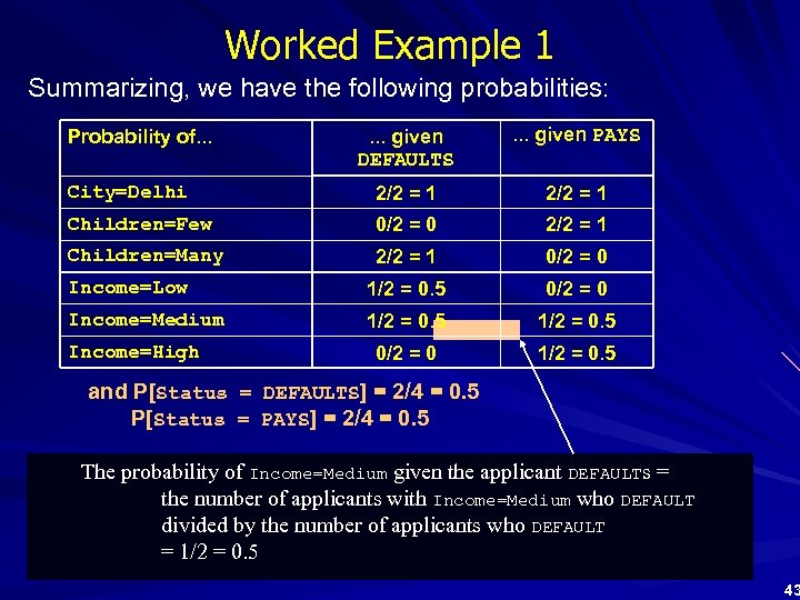 Worked Example 1 Summarizing, we have the following probabilities: . . . given DEFAULTS . . . given PAYS City=Delhi 2/2 = 1 Children=Few 0/2 = 0 2/2 = 1 Children=Many 2/2 = 1 0/2 = 0 Income=Low 1/2 = 0. 5 0/2 = 0 Income=Medium 1/2 = 0. 5 0/2 = 0 1/2 = 0. 5 Probability of. . . Income=High and P[Status = DEFAULTS] = 2/4 = 0. 5 P[Status = PAYS] = 2/4 = 0. 5 The probability of Income=Medium given the applicant DEFAULTs = the number of applicants with Income=Medium who DEFAULT divided by the number of applicants who DEFAULT = 1/2 = 0. 5 43
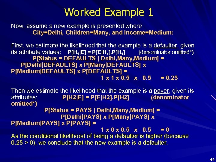 Worked Example 1 Now, assume a new example is presented where City=Delhi, Children=Many, and Income=Medium: First, we estimate the likelihood that the example is a defaulter, given its attribute values: P[H 1|E] = P[E|H 1]. P[H 1] (denominator omitted*) P[Status = DEFAULTS | Delhi, Many, Medium] = P[Delhi|DEFAULTS] x P[Many|DEFAULTS] x P[Medium|DEFAULTS] x P[DEFAULTS] = 1 x 0. 5 = 0. 25 Then we estimate the likelihood that the example is a payer, given its attributes: P[H 2|E] = P[E|H 2]. P[H 2] (denominator omitted*) P[Status = PAYS | Delhi, Many, Medium] = P[Delhi|PAYS] x P[Many|PAYS] x P[Medium|PAYS] x P[PAYS] = 1 x 0. 5 =0 As the conditional likelihood of being a defaulter is higher (because 0. 25 > 0), we conclude that the new example is a defaulter. 44
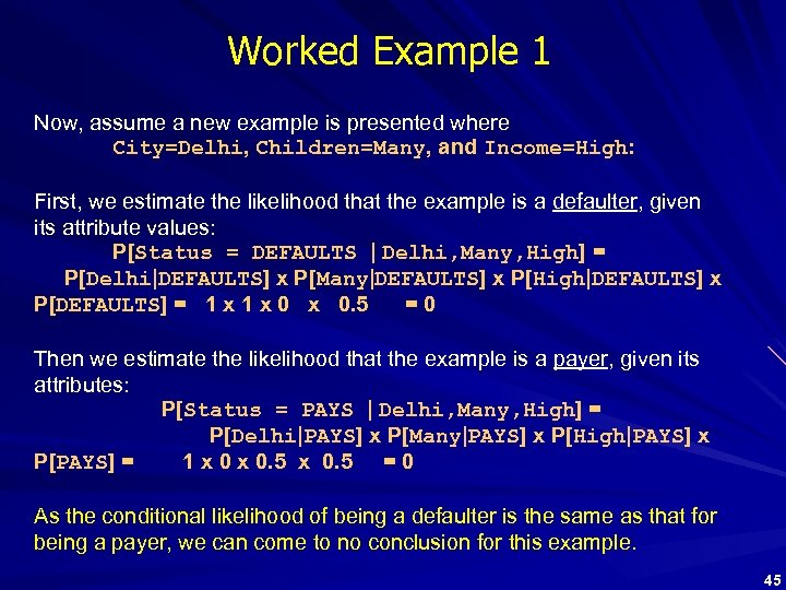 Worked Example 1 Now, assume a new example is presented where City=Delhi, Children=Many, and Income=High: First, we estimate the likelihood that the example is a defaulter, given its attribute values: P[Status = DEFAULTS | Delhi, Many, High] = P[Delhi|DEFAULTS] x P[Many|DEFAULTS] x P[High|DEFAULTS] x P[DEFAULTS] = 1 x 0 x 0. 5 =0 Then we estimate the likelihood that the example is a payer, given its attributes: P[Status = PAYS | Delhi, Many, High] = P[Delhi|PAYS] x P[Many|PAYS] x P[High|PAYS] x P[PAYS] = 1 x 0. 5 = 0 As the conditional likelihood of being a defaulter is the same as that for being a payer, we can come to no conclusion for this example. 45
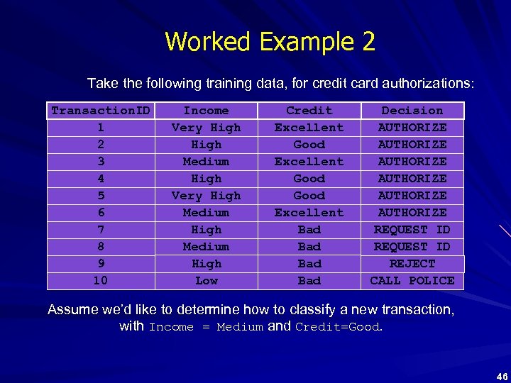 Worked Example 2 Take the following training data, for credit card authorizations: Transaction. ID 1 2 3 4 5 6 7 8 9 10 Income Very High Medium High Low Credit Excellent Good Excellent Bad Bad Decision AUTHORIZE AUTHORIZE REQUEST ID REJECT CALL POLICE Assume we’d like to determine how to classify a new transaction, with Income = Medium and Credit=Good. 46
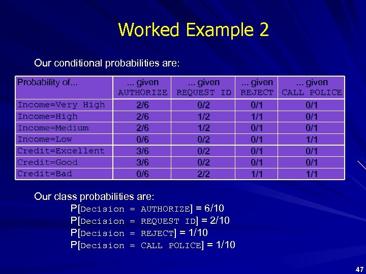 Worked Example 2 Our conditional probabilities are: Probability of. . . Income=Very High Income=Medium Income=Low Credit=Excellent Credit=Good Credit=Bad . . . given AUTHORIZE REQUEST ID REJECT CALL POLICE 2/6 0/2 0/1 2/6 1/2 1/1 0/1 2/6 1/2 0/1 0/6 0/2 0/1 1/1 3/6 0/2 0/1 0/1 0/6 2/2 1/1 Our class probabilities are: P[Decision = AUTHORIZE] = 6/10 P[Decision = REQUEST ID] = 2/10 P[Decision = REJECT] = 1/10 P[Decision = CALL POLICE] = 1/10 47
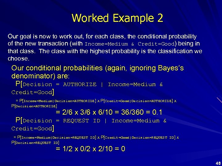 Worked Example 2 Our goal is now to work out, for each class, the conditional probability of the new transaction (with Income=Medium & Credit=Good) being in that class. The class with the highest probability is the classification we choose. Our conditional probabilities (again, ignoring Bayes’s denominator) are: P[Decision = AUTHORIZE | Income=Medium & Credit=Good] = P[Income=Medium|Decision=AUTHORIZE ] x P[Credit=Good|Decision=AUTHORIZE ] x P[Decision=AUTHORIZE ] = 2/6 x 3/6 x 6/10 = 36/360 = 0. 1 P[Decision = REQUEST ID | Income=Medium & Credit=Good] = P[Income=Medium|Decision=REQUEST ID ] x P[Credit=Good|Decision=REQUEST ID ] x P[Decision=REQUEST ID ] = 1/2 x 0/2 x 2/10 = 0 48
![Worked Example 2 P[Decision = REJECT | Income=Medium & Credit=Good] = P[Income=Medium|Decision=REJECT] x P[Credit=Good|Decision=REJECT] Worked Example 2 P[Decision = REJECT | Income=Medium & Credit=Good] = P[Income=Medium|Decision=REJECT] x P[Credit=Good|Decision=REJECT]](https://present5.com/presentation/a1ffdf92f322d4a3495126c35a1c384d/image-49.jpg) Worked Example 2 P[Decision = REJECT | Income=Medium & Credit=Good] = P[Income=Medium|Decision=REJECT] x P[Credit=Good|Decision=REJECT] x P[Decision=REJECT] = 0/1 x 1/10 = 0 P[Decision = CALL POLICE | Income=Medium & Credit=Good] = P[Income=Medium|Decision=CALL POLICE] x P[Credit=Good|Decision=CALL POLICE] x P[Decision=CALL POLICE] = 0/1 x 1/10 = 0 The highest of these probabilities is the first, so we conclude that the decision for our new transaction should be AUTHORIZE. 49
Worked Example 2 P[Decision = REJECT | Income=Medium & Credit=Good] = P[Income=Medium|Decision=REJECT] x P[Credit=Good|Decision=REJECT] x P[Decision=REJECT] = 0/1 x 1/10 = 0 P[Decision = CALL POLICE | Income=Medium & Credit=Good] = P[Income=Medium|Decision=CALL POLICE] x P[Credit=Good|Decision=CALL POLICE] x P[Decision=CALL POLICE] = 0/1 x 1/10 = 0 The highest of these probabilities is the first, so we conclude that the decision for our new transaction should be AUTHORIZE. 49
 Weaknesses • Naive Bayes assumes that variables are equally important and that they are independent which is often not the case in practice. • Naive Bayes is damaged by the inclusion of redundant (strongly dependent) attributes. e. g. if people with high income have expensive houses, then including both income and house-price in the model would unfairly multiply the effect of having low income. • Sparse data: If some attribute values are not present in the data, then a zero probability for P[E|H] might exist. This would lead P[H|E] to be zero no matter how high P[E|H] is for other attribute values. Small positive values which estimate the so-called ‘prior probabilities’ are often used to correct this. 50
 Classification Using Distance Place items in class to which they are “closest”. Must determine distance between an item and a class. n Classes represented by – Centroid: Central value. – Medoid: Representative point. – Individual points Algorithm: KNN
 K Nearest Neighbor (KNN): Training set includes classes. Examine K items near item to be classified. New item placed in class with the most number of close items. O(q) for each tuple to be classified. (Here q is the size of the training set. )
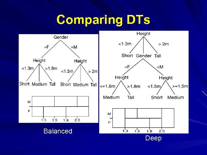
 Classification Using Decision Trees Partitioning based: Divide search space into rectangular regions. Tuple placed into class based on the region within which it falls. DT approaches differ in how the tree is built: DT Induction Internal nodes associated with attribute and arcs with values for that attribute. Algorithms: ID 3, C 4. 5, CART
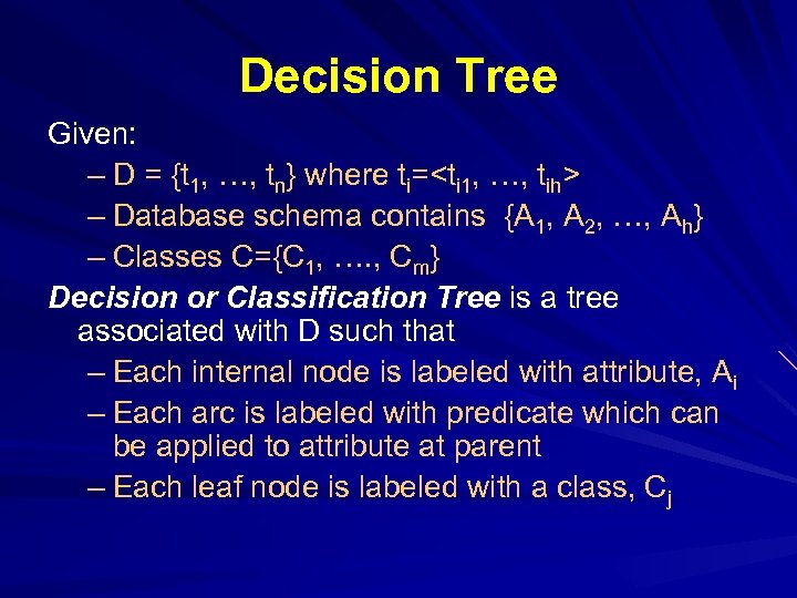 Decision Tree Given: – D = {t 1, …, tn} where ti=
 Comparing DTs Balanced Deep
 DT Issues Choosing Splitting Attributes Ordering of Splitting Attributes Splits Tree Structure Stopping Criteria Training Data Pruning
 DECISION TREES An internal node represents a test on an attribute. A branch represents an outcome of the test, e. g. , Color=red. A leaf node represents a class label or class label distribution. At each node, one attribute is chosen to split training examples into distinct classes as much as possible A new case is classified by following a matching path to a leaf node.
 Training Set
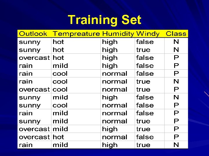
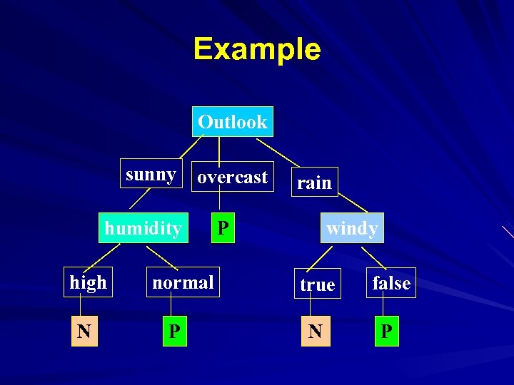 Example Outlook sunny overcast humidity high N normal P rain windy P true false N P
 Building Decision Tree Top-down tree construction – At start, all training examples are at the root. – Partition the examples recursively by choosing one attribute each time. Bottom-up tree pruning – Remove subtrees or branches, in a bottom-up manner, to improve the estimated accuracy on new cases. Use of decision tree: Classifying an unknown sample – Test the attribute values of the sample against the decision tree
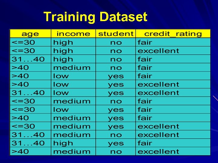 Training Dataset
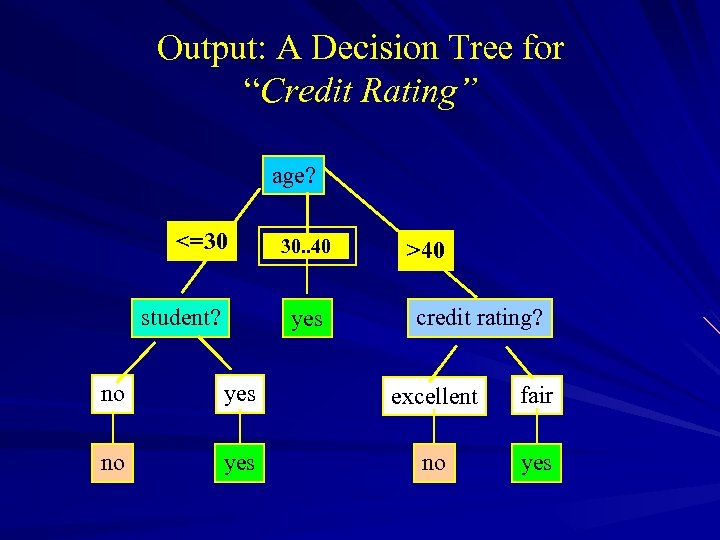 Output: A Decision Tree for “Credit Rating” age? <=30 student? overcast 30. . 40 yes >40 credit rating? no yes excellent fair no yes
 Algorithm for Decision Tree Induction Basic algorithm (a greedy algorithm) – Tree is constructed in a top-down recursive divide-andconquer manner – At start, all the training examples are at the root – Attributes are categorical – Examples are partitioned recursively based on selected attributes – Test attributes are selected on the basis of a heuristic or statistical measure (e. g. , information gain) Conditions for stopping partitioning – All samples for a given node belong to the same class – There are no remaining attributes for further partitioning – majority voting is employed for classifying the leaf – There are no samples left
 Choosing the Splitting Attribute At each node, available attributes are evaluated on the basis of separating the classes of the training examples. A Goodness function is used for this purpose. Typical goodness functions: – information gain (ID 3/C 4. 5) – information gain ratio – gini index
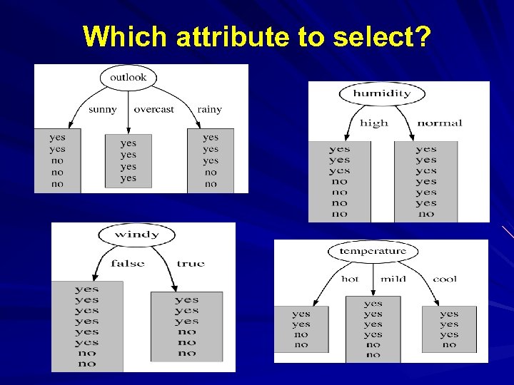 Which attribute to select?
 A criterion for attribute selection Which is the best attribute? – The one which will result in the smallest tree – Heuristic: choose the attribute that produces the “purest” nodes Popular impurity criterion: information gain – Information gain increases with the average purity of the subsets that an attribute produces Strategy: choose attribute that results in greatest information gain
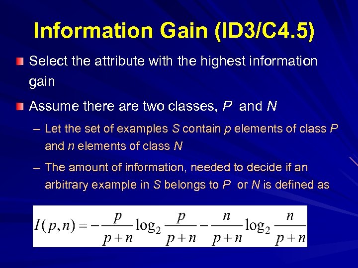 Information Gain (ID 3/C 4. 5) Select the attribute with the highest information gain Assume there are two classes, P and N – Let the set of examples S contain p elements of class P and n elements of class N – The amount of information, needed to decide if an arbitrary example in S belongs to P or N is defined as
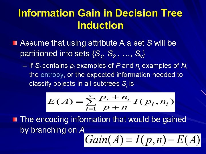 Information Gain in Decision Tree Induction Assume that using attribute A a set S will be partitioned into sets {S 1, S 2 , …, Sv} – If Si contains pi examples of P and ni examples of N, the entropy, or the expected information needed to classify objects in all subtrees Si is The encoding information that would be gained by branching on A
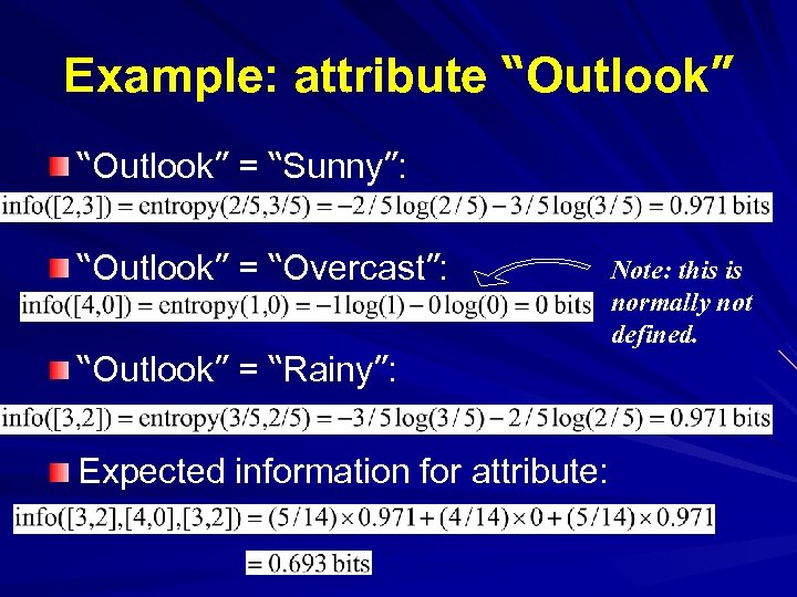 Example: attribute “Outlook” = “Sunny”: “Outlook” = “Overcast”: “Outlook” = “Rainy”: Expected information for attribute: Note: this is normally not defined.
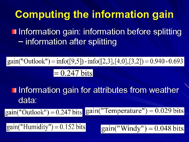 Computing the information gain Information gain: information before splitting – information after splitting Information gain for attributes from weather data:
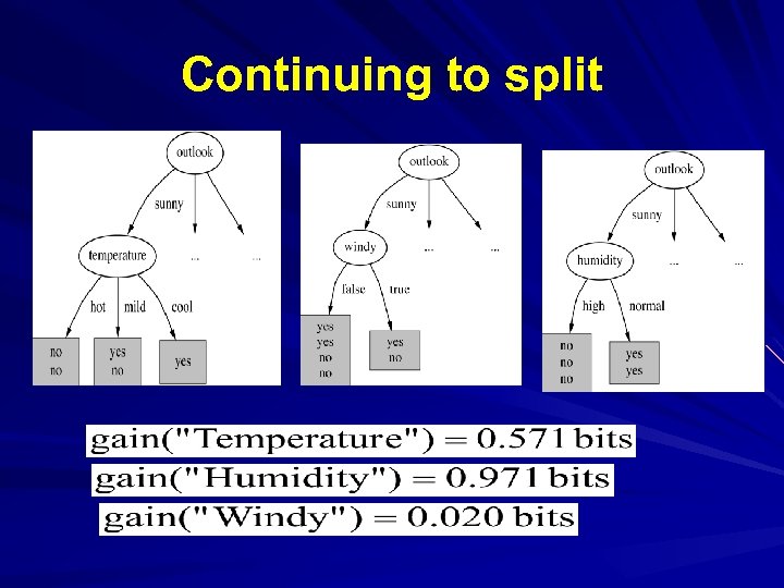 Continuing to split
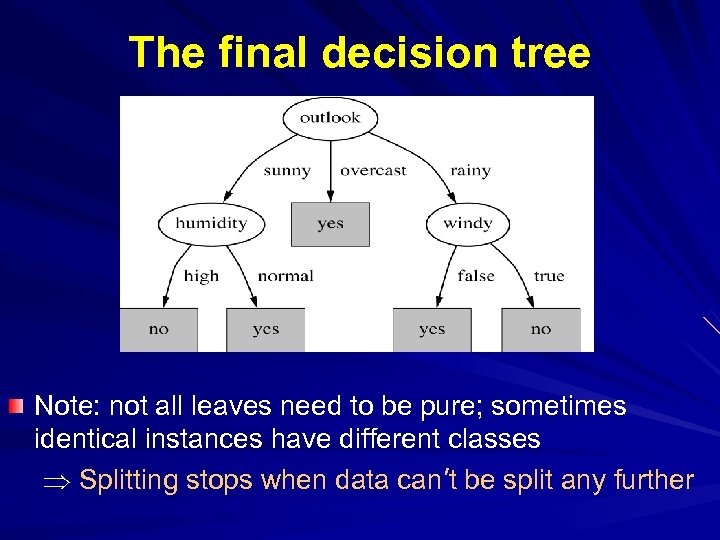 The final decision tree Note: not all leaves need to be pure; sometimes identical instances have different classes Splitting stops when data can’t be split any further
 Highly-branching attributes Problematic: attributes with a large number of values (extreme case: ID code) Subsets are more likely to be pure if there is a large number of values Information gain is biased towards choosing attributes with a large number of values This may result in overfitting (selection of an attribute that is non-optimal for prediction) Another problem: fragmentation
 The gain ratio Gain ratio: a modification of the information gain that reduces its bias on high-branch attributes Gain ratio takes number and size of branches into account when choosing an attribute – It corrects the information gain by taking the intrinsic information of a split into account – Also called split ratio Intrinsic information: entropy of distribution of instances into branches – (i. e. how much info do we need to tell which branch an instance belongs to)
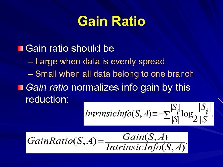 Gain Ratio Gain ratio should be – Large when data is evenly spread – Small when all data belong to one branch Gain ratio normalizes info gain by this reduction:
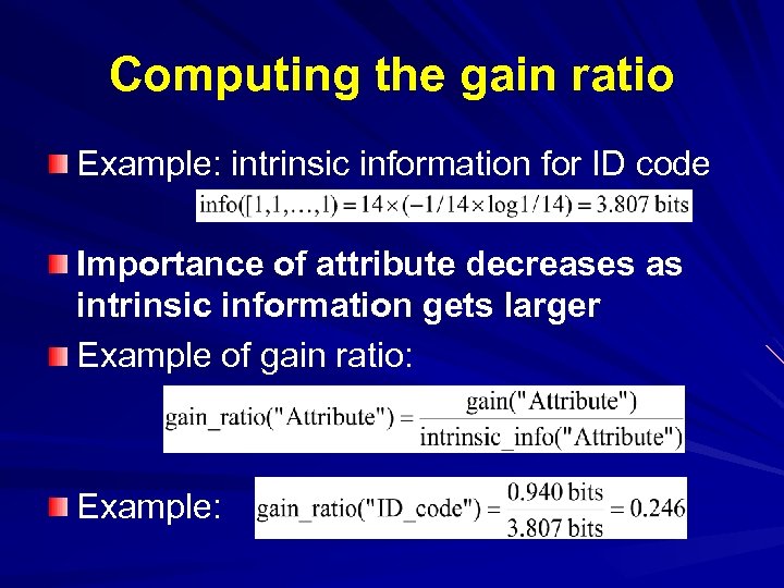 Computing the gain ratio Example: intrinsic information for ID code Importance of attribute decreases as intrinsic information gets larger Example of gain ratio: Example:
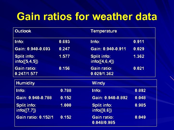 Gain ratios for weather data Outlook Temperature Info: 0. 693 Info: 0. 911 Gain: 0. 940 -0. 693 0. 247 Gain: 0. 940 -0. 911 0. 029 Split info: info([5, 4, 5]) 1. 577 Split info: info([4, 6, 4]) 1. 362 Gain ratio: 0. 247/1. 577 0. 156 Gain ratio: 0. 029/1. 362 0. 021 Humidity Windy Info: 0. 788 Info: 0. 892 Gain: 0. 940 -0. 788 0. 152 Gain: 0. 940 -0. 892 0. 048 Split info: info([7, 7]) 1. 000 Split info: info([8, 6]) 0. 985 Gain ratio: 0. 152/1 0. 152 Gain ratio: 0. 048/0. 985 0. 049
 Classification Using Rules Perform classification using If-Then rules Classification Rule: r =
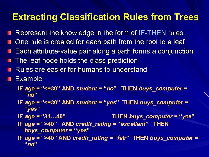 Extracting Classification Rules from Trees Represent the knowledge in the form of IF-THEN rules One rule is created for each path from the root to a leaf Each attribute-value pair along a path forms a conjunction The leaf node holds the class prediction Rules are easier for humans to understand Example IF age = “<=30” AND student = “no” THEN buys_computer = “no” IF age = “<=30” AND student = “yes” THEN buys_computer = “yes” IF age = “ 31… 40” THEN buys_computer = “yes” IF age = “>40” AND credit_rating = “excellent” THEN buys_computer = “yes” IF age = “>40” AND credit_rating = “fair” THEN buys_computer = “no”
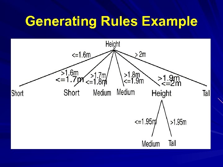 Generating Rules Example
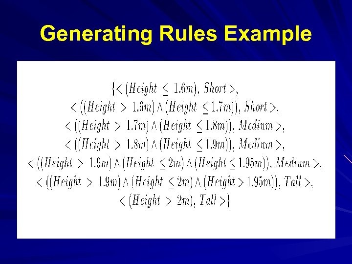 Generating Rules Example
 Avoid Overfitting in Classification The generated tree may overfit the training data – Too many branches, some may reflect anomalies due to noise or outliers – Result is in poor accuracy for unseen samples Two approaches to avoid overfitting – Prepruning: Halt tree construction early—do not split a node if this would result in the goodness measure falling below a threshold Difficult to choose an appropriate threshold – Postpruning: Remove branches from a “fully grown” tree—get a sequence of progressively pruned trees Use a set of data different from the training data to decide which is the “best pruned tree”
 Approaches to Determine the Final Tree Size Separate training (2/3) and testing (1/3) sets Use cross validation, e. g. , 10 -fold cross validation Use all the data for training – but apply a statistical test (e. g. , chi-square) to estimate whether expanding or pruning a node may improve the entire distribution Use minimum description length (MDL) principle: – halting growth of the tree when the encoding is minimized
 Enhancements to basic decision tree induction Allow for continuous-valued attributes – Dynamically define new discrete-valued attributes that partition the continuous attribute value into a discrete set of intervals Handle missing attribute values – Assign the most common value of the attribute – Assign probability to each of the possible values Attribute construction – Create new attributes based on existing ones that are sparsely represented – This reduces fragmentation, repetition, and replication
 Decision Tree vs. Rules Tree has implied order in which splitting is performed. Tree created based on looking at all classes. Rules have no ordering of predicates. Only need to look at one class to generate its rules.


