Data-Driven Batch Scheduling John Bent Ph D Oral

Data-Driven Batch Scheduling John Bent Ph. D. Oral Exam Department of Computer Sciences University of Wisconsin, Madison May 31, 2005

Batch Computing Highly successful, widely-deployed technology • Frequently used across the sciences • As well as in video production, document processing, data mining, financial services, graphics rendering Evolved into much more than a job queue • • Manages multiple distributed resources Handles complex job dependencies Checkpoints and migrates running jobs Enables transparent remote execution Environmental transparency is becoming problematic

Problem with Environmental Transparency Emerging trends • • Data sets are getting larger [Roselli 00, Zadok 04, LHC@CERN] Data growth outpacing increase in processing ability [Gray 03] More wide-area resources are available [Foster 01, Thain 04] Users push successful technology beyond design [Wall 02] Batch schedulers are CPU-centric • • Ignore data dependencies Data movement happens as a side-effect of job placement Great for compute-intensive workloads executing locally Horrible for data-intensive workloads executing remotely How to run data-intensive workloads remotely?

Approaches to Remote Execution Direct I/O: Direct remote data access • Simple and reliable • Large throughput hit Prestaging Data: Manipulating environment • Allows remote execution without performance hit • High user burden • Fault tolerance, restarts are difficult Distributed File Systems: AFS, NFS, etc. • Designed for wide-area networks and sharing • Infeasible across autonomous domains • Policies not appropriate for batch workloads

Common Fundamental Problem Layers upon CPU-centric scheduling Data planning external to the scheduler • “Second class citizen in batch scheduling” Data-aware scheduling policies needed • Knowledge of I/O behavior of batch workloads • Support from the file system • Data-driven batch scheduler

Outline Intro Profiling data-intensive batch workloads File system support Data-driven scheduling Conclusions and contributions

Selecting Workloads to Profile General characteristics of batch workloads? Select a representative suite of workloads • • BLAST IBIS CMS Hartree-Fock Nautilus AMANDA SETI@home biology ecology physics chemistry molecular dynamics astrophysics astronomy

Key Observation: Batch-Pipeline Workloads consist of many processes • Complex job and data dependencies • Three types of data and data sharing Vertical relationships: Pipelines • Processes often are vertically dependent • Output of parent becomes input to child Horizontal relationships: Batches • Users often submit multiple pipelines • May be read sharing across siblings

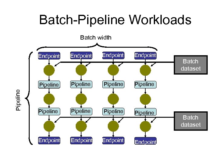
Batch-Pipeline Workloads Batch width Endpoint Pipeline Endpoint Pipeline Pipeline Endpoint Batch dataset

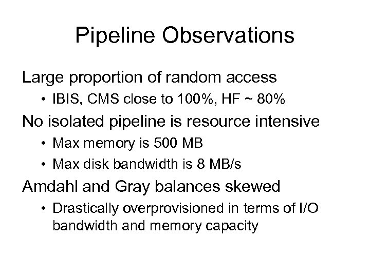
Pipeline Observations Large proportion of random access • IBIS, CMS close to 100%, HF ~ 80% No isolated pipeline is resource intensive • Max memory is 500 MB • Max disk bandwidth is 8 MB/s Amdahl and Gray balances skewed • Drastically overprovisioned in terms of I/O bandwidth and memory capacity

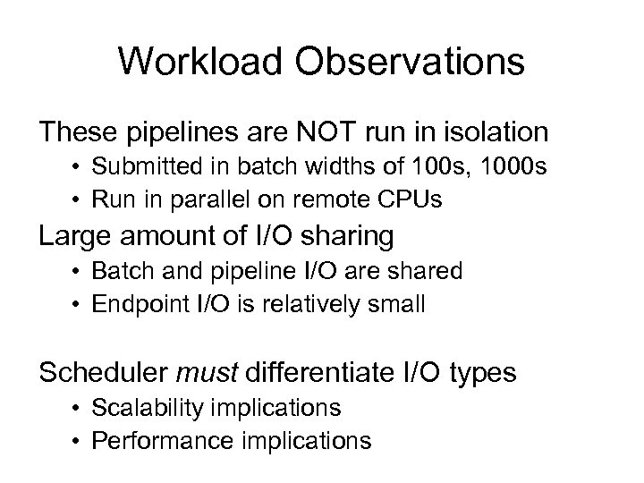
Workload Observations These pipelines are NOT run in isolation • Submitted in batch widths of 100 s, 1000 s • Run in parallel on remote CPUs Large amount of I/O sharing • Batch and pipeline I/O are shared • Endpoint I/O is relatively small Scheduler must differentiate I/O types • Scalability implications • Performance implications

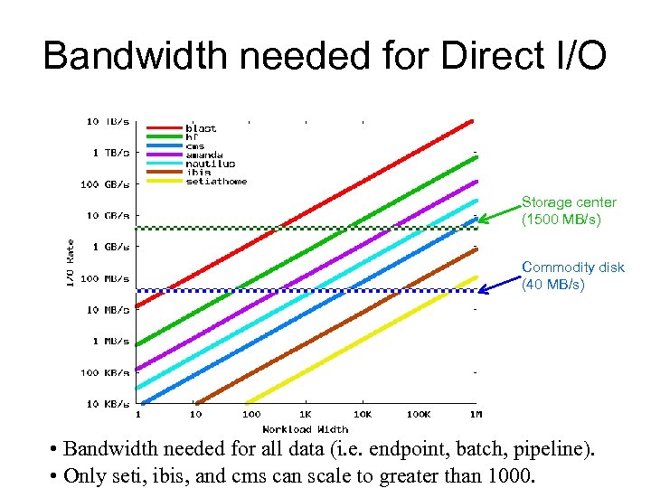
Bandwidth needed for Direct I/O Storage center (1500 MB/s) Commodity disk (40 MB/s) • Bandwidth needed for all data (i. e. endpoint, batch, pipeline). • Only seti, ibis, and cms can scale to greater than 1000.

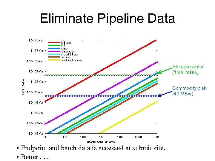
Eliminate Pipeline Data Storage center (1500 MB/s) Commodity disk (40 MB/s) • Endpoint and batch data is accessed at submit site. • Better. . .

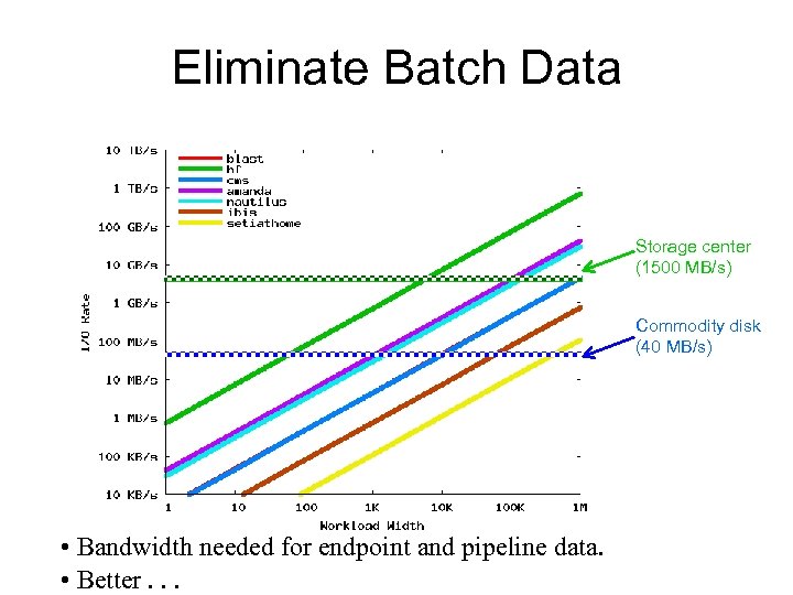
Eliminate Batch Data Storage center (1500 MB/s) Commodity disk (40 MB/s) • Bandwidth needed for endpoint and pipeline data. • Better. . .

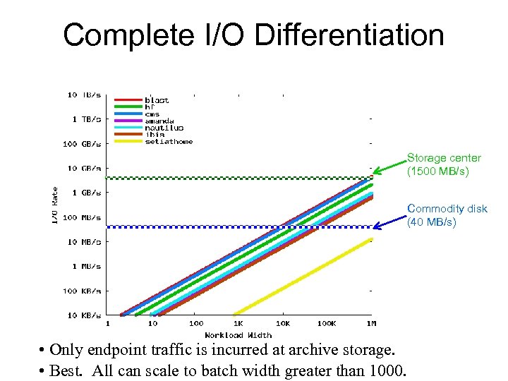
Complete I/O Differentiation Storage center (1500 MB/s) Commodity disk (40 MB/s) • Only endpoint traffic is incurred at archive storage. • Best. All can scale to batch width greater than 1000.

Outline Intro Profiling data-intensive batch workloads File system support • Develop new distributed file system: BAD-FS • Develop capacity-aware scheduler • Evaluate against CPU-centric scheduling Data-driven scheduling Conclusions and contributions

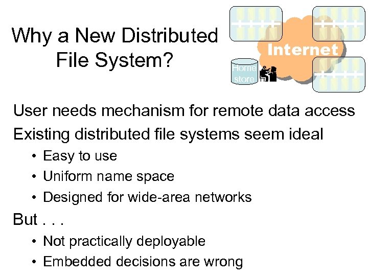
Why a New Distributed File System? Internet Home store User needs mechanism for remote data access Existing distributed file systems seem ideal • Easy to use • Uniform name space • Designed for wide-area networks But. . . • Not practically deployable • Embedded decisions are wrong

Existing DFS’s make bad decisions Caching • Must guess what and how to cache Consistency • Output: Must guess when to commit • Input: Needs mechanism to invalidate cache Replication • Must guess what to replicate

BAD-FS makes good decisions Removes the guesswork • Scheduler has detailed workload knowledge • Storage layer allows external control • Scheduler makes informed storage decisions Retains simplicity and elegance of DFS • Uniform name space • Location transparency Practical and deployable

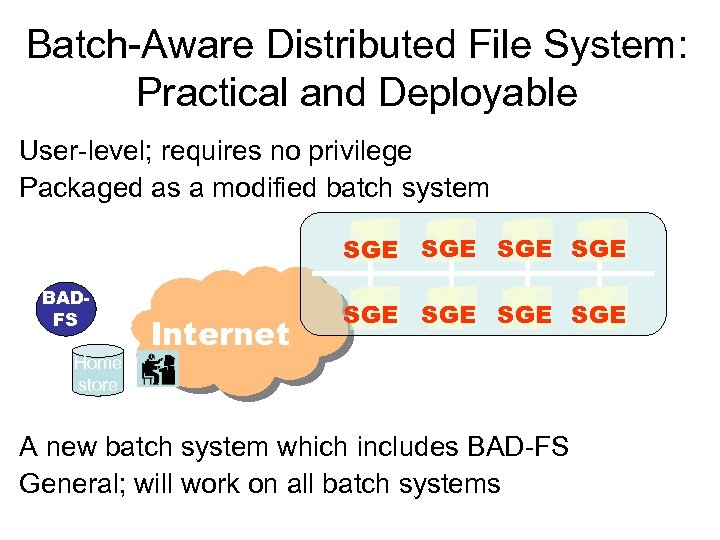
Batch-Aware Distributed File System: Practical and Deployable User-level; requires no privilege Packaged as a modified batch system SGE SGE BADFS Home store Internet SGE SGE A new batch system which includes BAD-FS General; will work on all batch systems

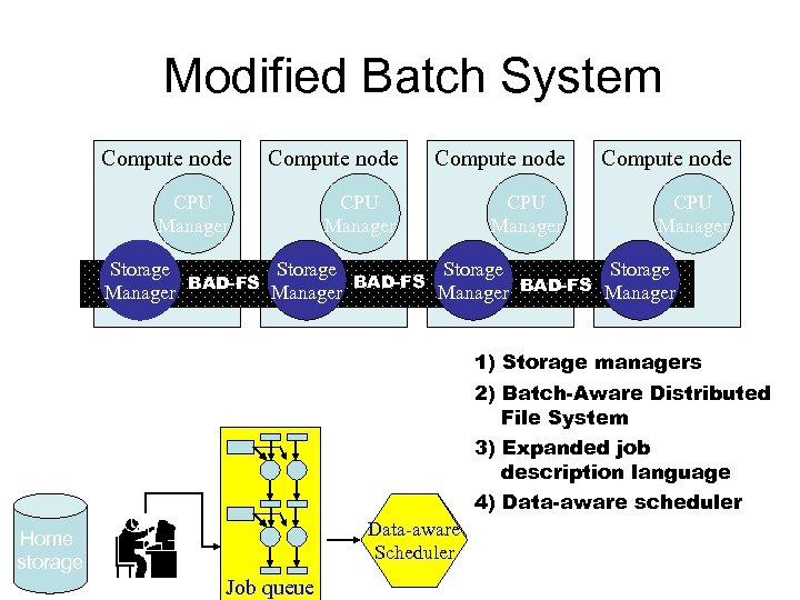
Modified Batch System Compute node CPU Manager Storage BAD-FS Manager BAD-FS Manager 1) Storage managers 2) Batch-Aware Distributed File System 3) Expanded job description language Home storage 1 2 3 4 Job queue 4) Data-aware scheduler Data-aware Scheduler

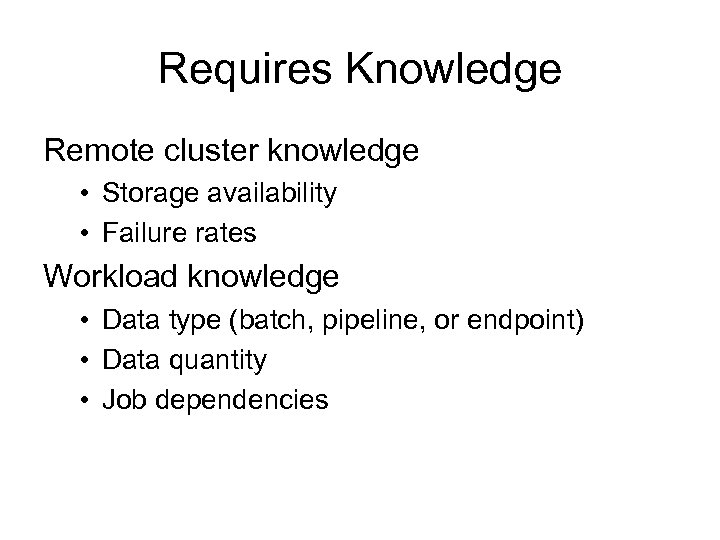
Requires Knowledge Remote cluster knowledge • Storage availability • Failure rates Workload knowledge • Data type (batch, pipeline, or endpoint) • Data quantity • Job dependencies

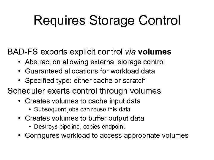
Requires Storage Control BAD-FS exports explicit control via volumes • Abstraction allowing external storage control • Guaranteed allocations for workload data • Specified type: either cache or scratch Scheduler exerts control through volumes • Creates volumes to cache input data • Subsequent jobs can reuse this data • Creates volumes to buffer output data • Destroys pipeline, copies endpoint • Configures workload to access appropriate volumes

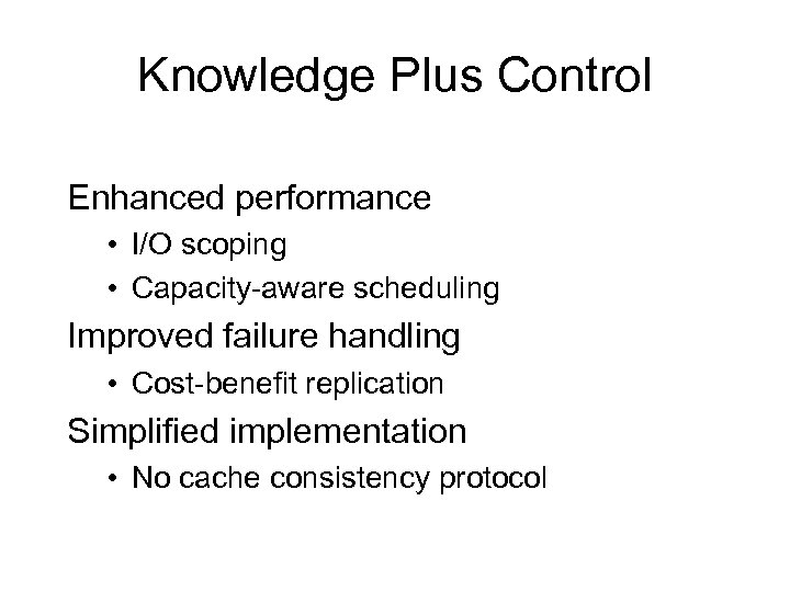
Knowledge Plus Control Enhanced performance • I/O scoping • Capacity-aware scheduling Improved failure handling • Cost-benefit replication Simplified implementation • No cache consistency protocol

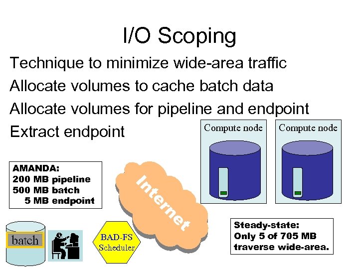
I/O Scoping Technique to minimize wide-area traffic Allocate volumes to cache batch data Allocate volumes for pipeline and endpoint Compute node Extract endpoint In et rn te AMANDA: 200 MB pipeline 500 MB batch 5 MB endpoint BAD-FS Scheduler Steady-state: Only 5 of 705 MB traverse wide-area.

Capacity-Aware Scheduling Technique to avoid over-allocations • Over-allocated batch data causes WAN thrashing • Over-allocated pipeline data causes write failures Scheduler has knowledge of • Storage availability • Storage usage within the workload Scheduler runs as many jobs as can fit

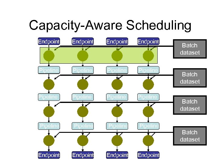
Capacity-Aware Scheduling Endpoint Pipeline Endpoint Pipeline Pipeline Batch dataset Pipeline Batch dataset Endpoint

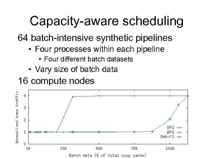
Capacity-aware scheduling 64 batch-intensive synthetic pipelines • Four processes within each pipeline • Four different batch datasets • Vary size of batch data 16 compute nodes

Improved failure handling Scheduler understands data semantics • Data is not just a collection of bytes • Losing data is not catastrophic • Output can be regenerated by rerunning jobs Cost-benefit replication • Replicates only data whose replication cost is cheaper than cost to rerun the job

Simplified implementation Data dependencies known Scheduler ensures proper ordering Build a distributed file system • With cooperative caching • But without a cache consistency protocol

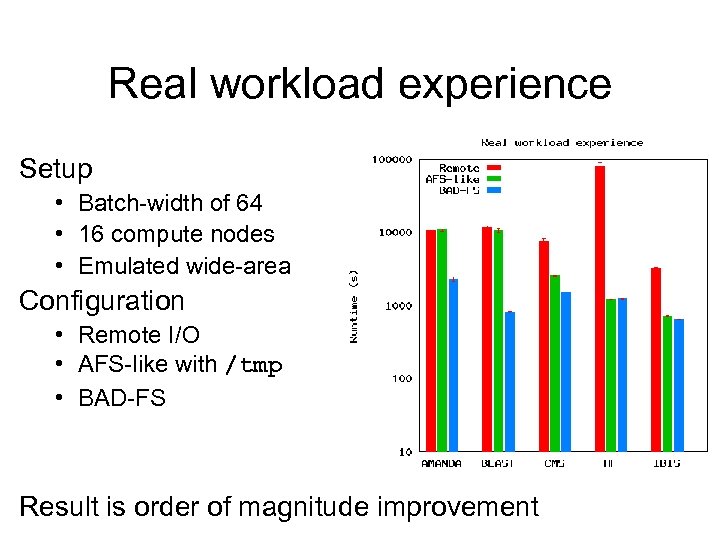
Real workload experience Setup • Batch-width of 64 • 16 compute nodes • Emulated wide-area Configuration • Remote I/O • AFS-like with /tmp • BAD-FS Result is order of magnitude improvement

Outline Intro Profiling data-intensive batch workloads File system support Data-driven scheduling • • • Codify simplifying assumptions Define data-driven scheduling policies Develop predictive analytical models Evaluate Discuss Conclusions and contributions

Simplifying Assumptions Predictive models • Only interested in relative (not absolute) accuracy Batch-pipeline workloads are “canonical” • Mostly uniform and homogeneous • Combine pipeline and endpoint data into private Environment • Assume homogeneous compute nodes Target scenario • Single workload on a single compute cluster

Predictive Accuracy: Choosing Relative over Absolute Develop predictive models to guide scheduler • Absolute accuracy not needed • Relative accuracy to select between different possible schedules Predictive model does not consider • • Latencies Disk bandwidths Buffer cache size or bandwidth Other “lower” characteristics such as buses, CPUs, etc Simplify model and retain relative predictive accuracy • These effects are more uniform across different possible schedules • Network and CPU utilization make largest difference The Trade-off? Loss of absolute accuracy

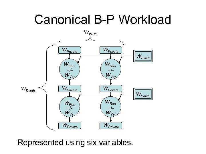
Canonical B-P Workload WWidth WPrivate WRun +/WVar WPrivate WDepth WPrivate Represented using six variables. WBatch

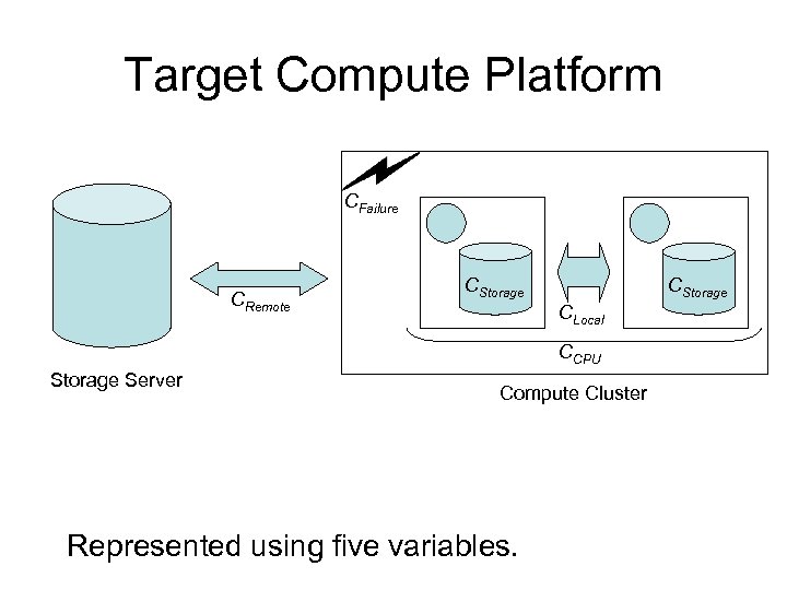
Target Compute Platform CFailure CRemote CStorage CLocal CCPU Storage Server Compute Cluster Represented using five variables.

Scheduling Objective Maximize throughput for user workloads Easy without data considerations • Run as many jobs as possible Potential problems with data considerations • WAN overutilization by resending batch data • Data barriers can reduce CPU utilization • Concurrency limits can reduce CPU utilization Need data-driven policies to avoid these problems

Five Scheduling Allocations Define allocations to avoid problems • • • All: Has no constraints; allows CPU-centric scheduling All. Batch: Avoids overutilizing WAN and barriers All. Private: Avoids concurrency limits Slice: Avoids overutilizing WAN Minimal: Attempts to maximize concurrency Each allocation might incur other problems Which problems are incurred by each?

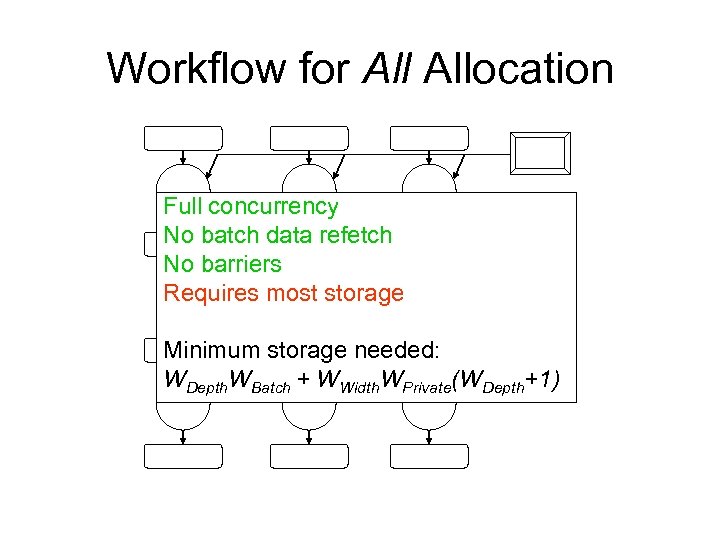
Workflow for Allocation Full concurrency No batch data refetch No barriers Requires most storage Minimum storage needed: WDepth. WBatch + WWidth. WPrivate(WDepth+1)

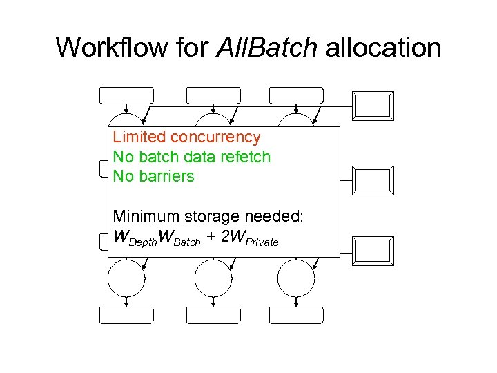
Workflow for All. Batch allocation Limited concurrency No batch data refetch No barriers Minimum storage needed: WDepth. WBatch + 2 WPrivate

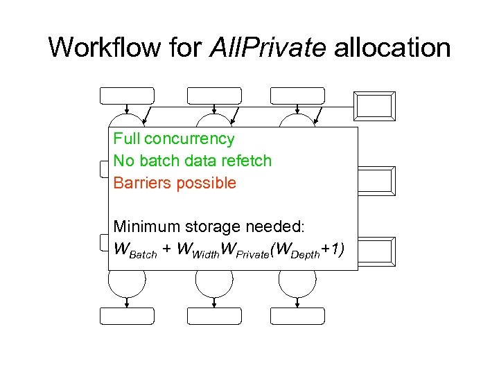
Workflow for All. Private allocation Full concurrency No batch data refetch Barriers possible Minimum storage needed: WBatch + WWidth. WPrivate(WDepth+1)

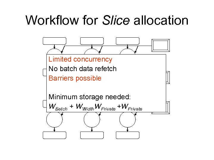
Workflow for Slice allocation Limited concurrency No batch data refetch Barriers possible Minimum storage needed: WBatch + WWidth. WPrivate +WPrivate

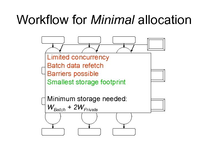
Workflow for Minimal allocation Limited concurrency Batch data refetch Barriers possible Smallest storage footprint Minimum storage needed: WBatch + 2 WPrivate

Selecting an allocation Multiple allocations may be possible • Dependent on WWidth and WDepth • Dependent of WBatch and WPrivate Which allocations are possible? Which possible allocation is preferrable?

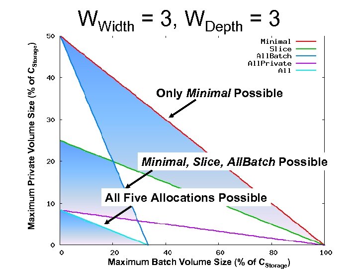
Maximum Private Volume Size (% of CStorage) WWidth = 3, WDepth = 3 Only Minimal Possible Minimal, Slice, All. Batch Possible All Five Allocations Possible Maximum Batch Volume Size (% of CStorage)

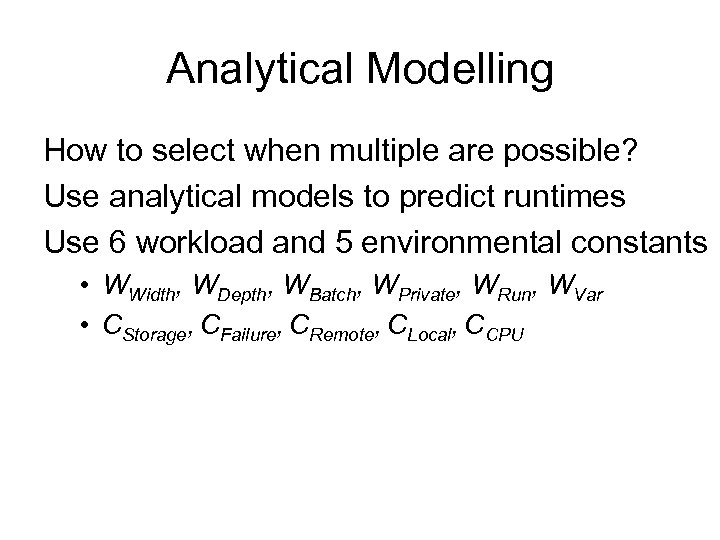
Analytical Modelling How to select when multiple are possible? Use analytical models to predict runtimes Use 6 workload and 5 environmental constants • WWidth, WDepth, WBatch, WPrivate, WRun, WVar • CStorage, CFailure, CRemote, CLocal, CCPU

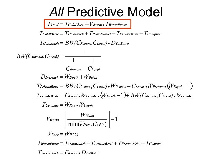
All Predictive Model

All. Batch Predictive Model

All. Private Predictive Model

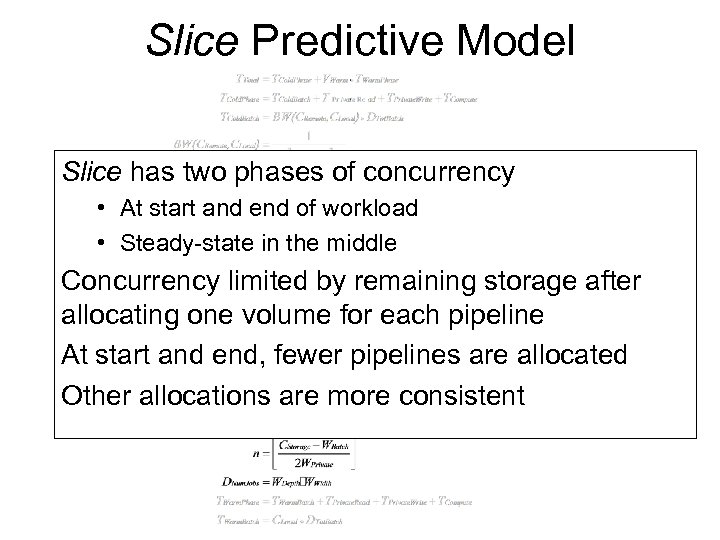
Slice Predictive Model Slice has two phases of concurrency • At start and end of workload • Steady-state in the middle Concurrency limited by remaining storage after allocating one volume for each pipeline At start and end, fewer pipelines are allocated Other allocations are more consistent

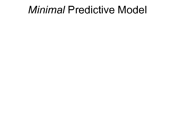
Minimal Predictive Model

Variables Used Workload Variables • WWidth and WDepth • WBatch and WPrivate • WRun and WVar Environmental Variables • CLocal and CRemote • CCPU and CStorage CFailure not considered in the models

Modelling Failure Effect Almost uniform effect across allocations • Estimate TTotal • Multiply by CFailure to estimate failed pipelines • Estimate TTotal for remaining failed pipelines Only one difference across allocations • For All and All. Batch, estimates for re-running failed pipelines do not include a “cold” phase

Evaluation Winnow the allocations Define three synthetic workloads • Batch-intensive, private-intensive, mixed Simulate workloads and allocations across • Workload variables (WBatch, etc) • Environmental variables (CFailure, etc) Compare modelled predictions with results

Winnowing the Allocations: Removing All and All. Private Remove All from consideration • Lacks constraint • No possible schedule results in problems • Scheduling is uninteresting Remove All. Private from consideration • Is a strict subset of Slice • When possible, Slice can run at full CPU utilization • No reason to prefer All. Private over Slice • All. Private more likely to suffer barriers • No benefit to holding onto “old” pipeline data

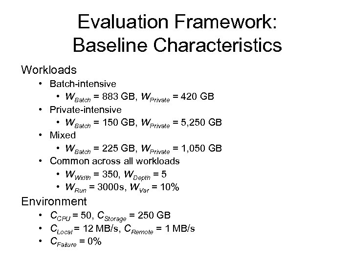
Evaluation Framework: Baseline Characteristics Workloads • Batch-intensive • WBatch = 883 GB, WPrivate = 420 GB • Private-intensive • WBatch = 150 GB, WPrivate = 5, 250 GB • Mixed • WBatch = 225 GB, WPrivate = 1, 050 GB • Common across all workloads • WWidth = 350, WDepth = 5 • WRun = 3000 s, WVar = 10% Environment • CCPU = 50, CStorage = 250 GB • CLocal = 12 MB/s, CRemote = 1 MB/s • CFailure = 0%

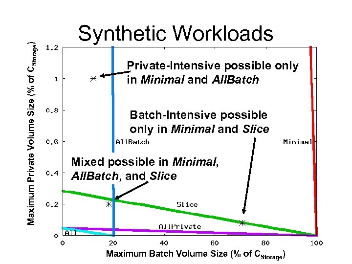
Maximum Private Volume Size (% of CStorage) Synthetic Workloads Private-Intensive possible only in Minimal and All. Batch-Intensive possible only in Minimal and Slice Mixed possible in Minimal, All. Batch, and Slice Maximum Batch Volume Size (% of CStorage)

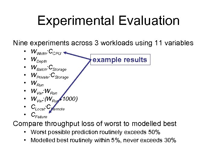
Experimental Evaluation Nine experiments across 3 workloads using 11 variables • • • WWidth: CCPU WDepth WBatch: CStorage WPrivate: CStorage WRun WVar: (WRun● 1000) CLocal: CRemote CFailure example results Compare throughput loss of worst to modelled best • Worst possible prediction routinely exceeds 50% • Modelled best routinely within 5%, never exceeds 30%

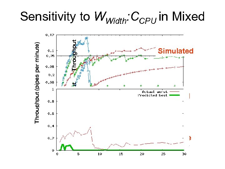
Throughput Simulated Throughput Loss Throughput (pipes per minute) Sensitivity to WWidth: CCPU in Mixed Modelled WWidth: CCPU Predictive accuracy

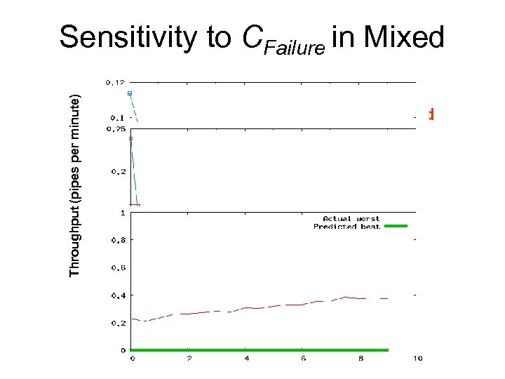
Throughput Simulated Throughput Loss Throughput (pipes per minute) Sensitivity to CFailure in Mixed Modelled CFailure Predictive accuracy

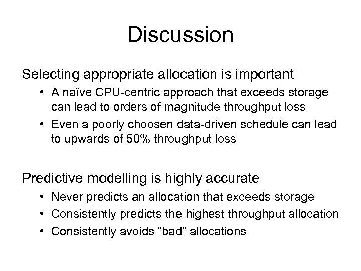
Discussion Selecting appropriate allocation is important • A naïve CPU-centric approach that exceeds storage can lead to orders of magnitude throughput loss • Even a poorly choosen data-driven schedule can lead to upwards of 50% throughput loss Predictive modelling is highly accurate • Never predicts an allocation that exceeds storage • Consistently predicts the highest throughput allocation • Consistently avoids “bad” allocations

What about non-canonical? Canonical scheduling still useful • Many workloads may be “almost” canonical • Canonical scheduling will work but might leave unnecessary pockets of CPU / storage • Similar to PBS which often elicits overly conservative runtime estimates Avoids deadlock or failures

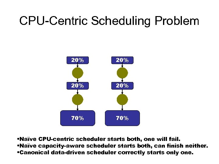
CPU-Centric Scheduling Problem 20% 20% 70% • Naïve CPU-centric scheduler starts both, one will fail. • Naïve capacity-aware scheduler starts both, can finish neither. • Canonical data-driven scheduler correctly starts only one.

Outline Intro Profiling data-intensive batch workloads File system support Data-driven scheduling Conclusions and contributions

Related Work Distributed file systems • GFS [Ghemawat 03] • P 2 P [Dahlin 94, Kubi 00, Muthitacharoen 02, Rowstron 01, Saito 02] • Untrusted storage nodes [Flinn 03] Data management in grid computing • Free. Loader [Vazhkudai 05] • Caching and locating batch data [Bell 03, Bent 05, Chervenak 02, Lamehehamedi 03, Park 03, Ranganathan 02, Romosan 05] • Stork [Kosar 04] Parallel scheduling • Gang scheduling with memory constraint [Batat 00] • Backfilling [Lifka 95] • Reserving non-dedicated resources [Snell 00] Query planning • LEO [Markl 03] • Proactive reoptimization [Babu 05]

Conclusions Batch computing is successful for a reason. • • Simple mechanism Easy to understand use Great need for it Works well But. The world is changing. • • Data sets are getting larger Increased availability of remote resources Existing approaches are fraught with problems CPU-centric scheduling is insufficient New data-driven policies are needed.

Contributions Profiling • Batch-pipeline workloads • Taxonomy to reason about workloads • Taxonomy to distinguish between data types • Data differentiation allows data-driven scheduling File system support • Transfer of explicit storage control • Batch scheduler dictates allocation, caching, replication • Order of magnitude improvement over CPU-centric Data-driven batch scheduling • Multiple allocations and scheduling policies • Predictive analytical model

End of Talk

Future Work Measurement Information • Collecting • Retrieving • Mitigating inaccuracies Multi-* Non-canonical Dynamic reallocation Checkpointing Partial results