Current work at UCL KCL Application

Current work at UCL & KCL

Application 2 Project aim: find the network of regions associated with pleasant and unpleasant stimuli and use this information to classify new stimuli (i. e. is the activation pattern to a new product closest to the pleasant, unpleasant or neutral pattern) We used f. MRI data from 16 healthy subjects viewing unpleasant, pleasant and neutral pictures.

Data Description Number of subjects: 16 Tasks: Viewing unpleasant and pleasant pictures (6 blocks of 7 scans) Pre-Processing Procedures • Realignment, normalization to standard space, spatial filter. • Mask to select voxels inside the brain. Training Examples • Mean volume per block Leave one-out-test • Training: 15 subjects • Test: 1 subject This procedure was repeated 16 times and the results (error rate) were averaged.

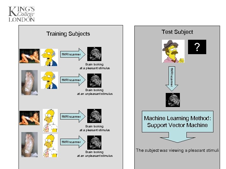Training Subjects Test Subject ? f. MRI scanner Brain looking at a pleasant stimulus Brain looking at an unpleasant stimulus f. MRI scanner Brain looking at a pleasant stimulus Machine Learning Method: Support Vector Machine f. MRI scanner Brain looking at an unpleasant stimulus The subject was viewing a pleasant stimuli

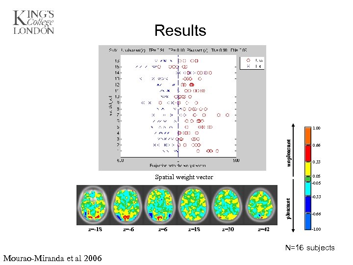Results unpleasant 1. 00 Spatial weight vector 0. 66 0. 33 0. 05 pleasant -0. 05 z=-18 z=-6 z=18 z=30 z=42 -0. 33 -0. 66 -1. 00 N=16 subjects Mourao-Miranda et al 2006

Application 3 • Project aim: discriminate depressed patients from healthy controls using their pattern of brain activation in response to emotional stimuli • We used f. MRI data from 19 free medication depressed patients vs. 19 healthy controls; • The f. MRI paradigm consisted of affective processing of sad facial stimuli with modulation of the intensity of the emotional expression (low, medium, and high intensity).

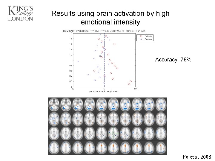Results using brain activation by high emotional intensity Accuracy=76% Fu et al 2008

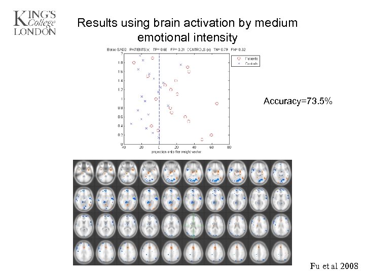Results using brain activation by medium emotional intensity Accuracy=73. 5% Fu et al 2008

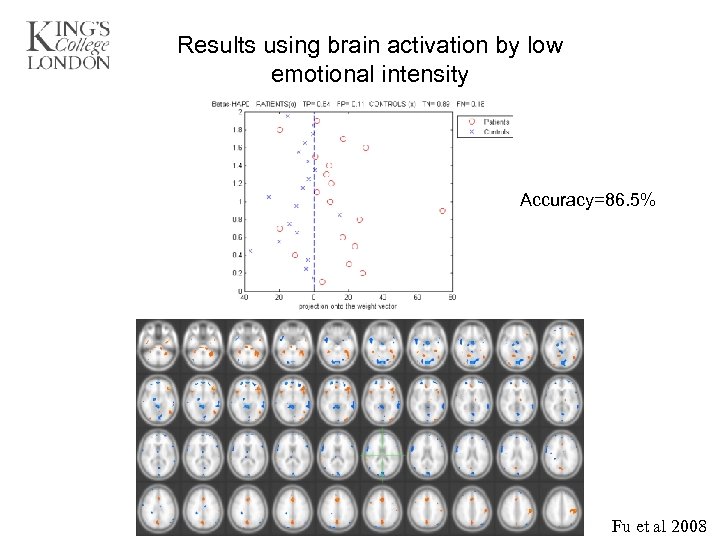Results using brain activation by low emotional intensity Accuracy=86. 5% Fu et al 2008

Wellcome Trust Grant Project title: A machine learning approach to the analysis of psychiatric neuroimaging data Aim: Develop mathematical models and tools for the application of novel machine learning techniques to the automated analysis of brain imaging data. Duration: 07/2009 -06/2014

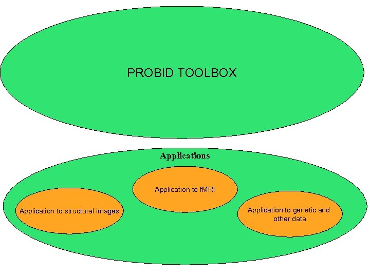Developments Data Representation & Feature Selections Categorical Classification SVM Probabilistic Classification GP PROBID TOOLBOX Outliers detection OCSVM Temporal based classification Multimodal Classification Correlation of different sources of information: KCCA Applications Application to f. MRI Application to structural images Application to genetic and other data

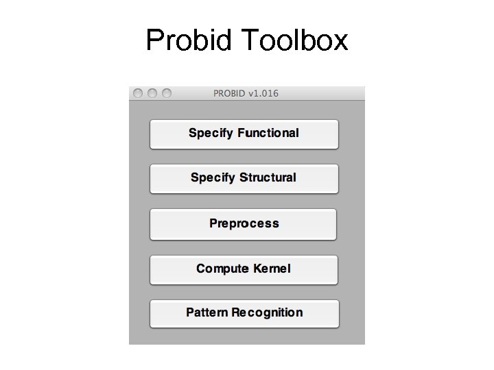
PROBID Toolbox Pattern Recognition of Brain Imaging Data

Development Team • Dr. Janaina Mourao-Miranda – Algorithm development • Andre Marquand – Graphical interface and algorithm development • Dr. Jane Rondina – Graphical interface and algorithm development • Dr. Vincent Giampietro – Algorithm development

Sponsors & Collaborators • • Professor John Shawe-Taylor, CSML, UCL Professor Steve Williams, IOP, KCL Professor Mick Brammer, IOP, KCL Professor Gareth Barker, IOP, KCL

Aim • Matlab toolbox optimized for group comparison and clinical research studies. • It provides: (1) an accessible interface to categorical (SVM) and probabilistic (Gaussian Process) pattern recognition algorithms; (2) a processing pipeline for most common neuroimaging data modalities (f. MRI, s. MRI, diffusion- and perfusion MRI and a text input module); (3) leave-one-subject (LOO) out cross-validation framework; (4) a permutation testing framework for robust significance testing.

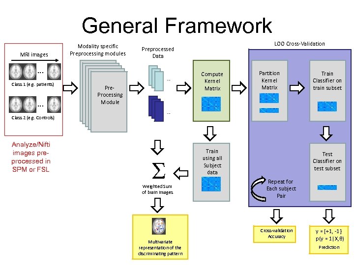General Framework MRI images . . . Class 1 (e. g. patients) . . . Modality specific Preprocessing modules Pre. Processing Pre. Processing Module Module . . . Compute Kernel Matrix Partition Kernel Matrix Train Classifier on train subset . . . Class 2 (e. g. Controls) Analyze/Nifti images preprocessed in SPM or FSL LOO Cross-Validation Preprocessed Data Σ Weighted Sum of brain images Multivariate representation of the discriminating pattern Train using all Subject data Test Classifier on test subset Repeat for Each subject Pair Cross-validation Accuracy y = {+1, -1} p(y = 1|X, θ) Prediction

Probid Toolbox

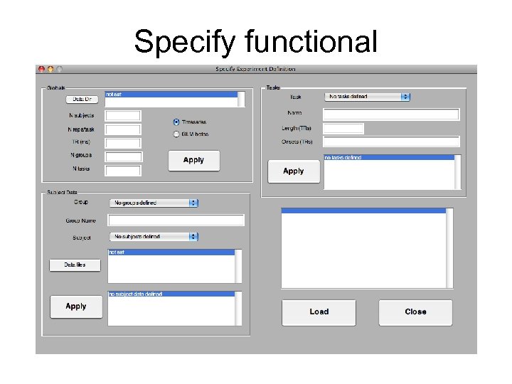Specify functional

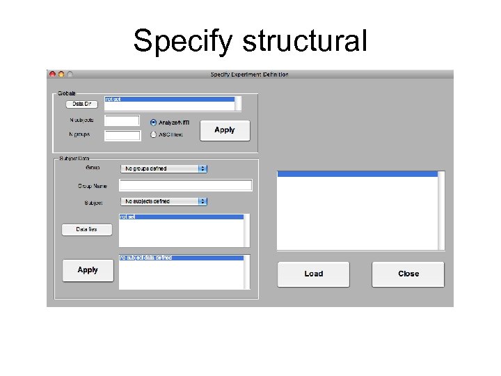Specify structural

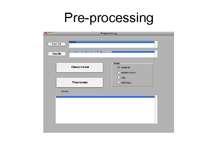Pre-processing

Pre-processing • f. MRI: – Detrend voxel time series; – Select parts of the time series correspondent to each experimental condition (accounting for the HRF delay). – Apply a mask to select voxels (whole brain or ROI) – Create pattern: • Single volumes • Mean volume • Spatiotemporal pattern

Pre-processing • Structural or GLM coefficients (f. MRI) – Apply a mask to select voxels (whole brain or ROI) – Create pattern: • Each volume represents one pattern • Perfusion – Apply a mask – Mean-centering data volumes within each subject to accommodate inter-subject differences in baseline signal.

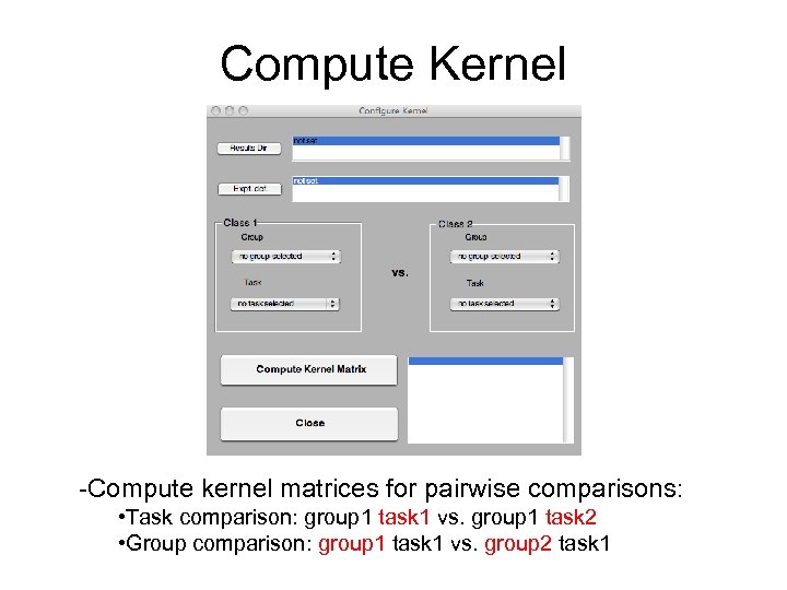Compute Kernel -Compute kernel matrices for pairwise comparisons: • Task comparison: group 1 task 1 vs. group 1 task 2 • Group comparison: group 1 task 1 vs. group 2 task 1

Kernel Matrix and Crossvalidation procedure • Pattern: – x 1=[x 1 … xv], v=number of features or voxels • Data matrix: – Dm, v = [x 1 … xm], m=number of examples • Linear kernel matrix: – K=DDT • For each LOO cross-validation iteration – Ktrain = K[index of training examples, index of training examples] – Ktest = K[index of test examples, index of training examples]

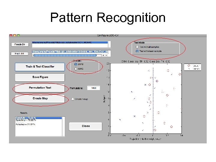Pattern Recognition

Classifiers Implemented • Support Vector Machine Classifier – LIBSVM toolbox – Linear Kernel – Parameter: • C=1 • Gaussian Process Classifier – GPML toolbox – Linear Covariance function – Parameters: • Bias (b) and regularization (l) (set automatically by the GPC framework using an empirical Bayesian approach, Marquand et al, in press)

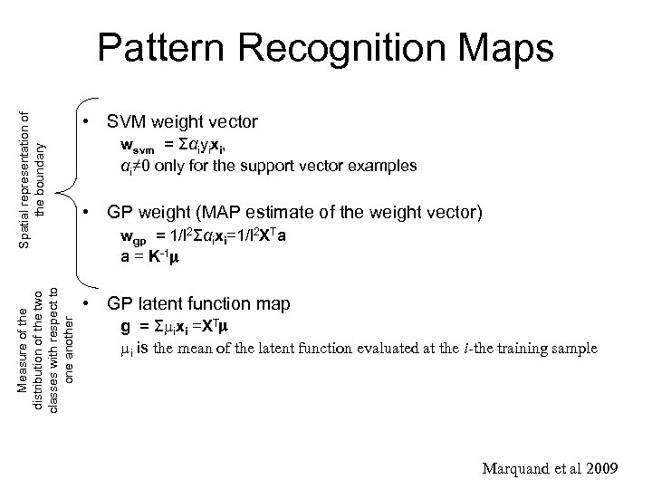Spatial representation of the boundary • SVM weight vector Measure of the distribution of the two classes with respect to one another Pattern Recognition Maps • GP latent function map wsvm = Σαiyixi, αi≠ 0 only for the support vector examples • GP weight (MAP estimate of the weight vector) wgp = 1/l 2Σαixi=1/l 2 XTa a = K-1 g = Σ ixi =XT i is the mean of the latent function evaluated at the i-the training sample Marquand et al 2009

On-going & Future Work • Outlier Detection: One-class SVM • Dynamic System models for classification • Multi-modal fusion • Power analysis for Pattern Recognition • Classification of Resting State f. MRI