CSI 5388 Topics in Machine Learning Inductive Learning

CSI 5388: Topics in Machine Learning Inductive Learning: A Review 1

Course Outline l Overview l Theory l Version Spaces l Decision Trees l Neural Networks 2

Inductive Learning : Overview l Different types of inductive learning: – Supervised Learning: The program attempts to infer an association between attributes and their inferred class. l Concept Learning l Classification – Unsupervised Learning: The program attempts to infer an association between attributes but no class is assigned. : l Reinforced learning. l Clustering l Discovery – Online vs. Batch Learning l We will focus on supervised learning in batch mode. 3

Inductive Inference Theory (1) l Given X the set of all examples. l A concept C is a subset of X. l A training example T is a subset of X such that some examples of T are elements of C (the positive examples) and some examples are not elements of C (the negative examples) 4

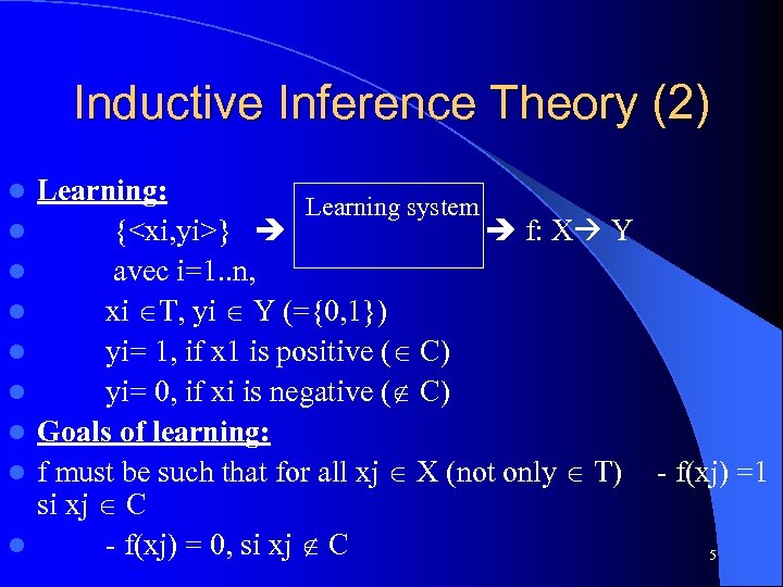Inductive Inference Theory (2) l l l l l Learning: Learning system {} f: X Y avec i=1. . n, xi T, yi Y (={0, 1}) yi= 1, if x 1 is positive ( C) yi= 0, if xi is negative ( C) Goals of learning: f must be such that for all xj X (not only T) - f(xj) =1 si xj C - f(xj) = 0, si xj C 5

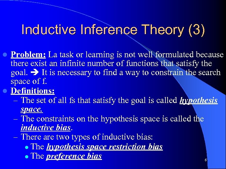Inductive Inference Theory (3) Problem: La task or learning is not well formulated because there exist an infinite number of functions that satisfy the goal. It is necessary to find a way to constrain the search space of f. l Definitions: – The set of all fs that satisfy the goal is called hypothesis space. – The constraints on the hypothesis space is called the inductive bias. – There are two types of inductive bias: l The hypothesis space restriction bias l The preference bias 6 l

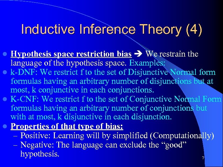Inductive Inference Theory (4) Hypothesis space restriction bias We restrain the language of the hypothesis space. Examples: l k-DNF: We restrict f to the set of Disjunctive Normal formulas having an arbitrary number of disjunctions but at most, k conjunctive in each conjunctions. l K-CNF: We restrict f to the set of Conjunctive Normal Form formulas having an arbitrary number of conjunctions but with at most, k disjunctive in each disjunction. l Properties of that type of bias: – Positive: Learning will by simplified (Computationally) – Negative: The language can exclude the “good” hypothesis. 7 l

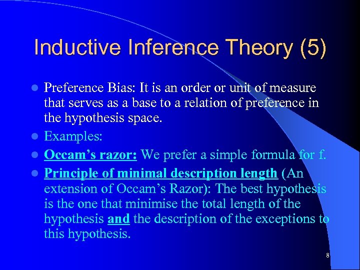Inductive Inference Theory (5) Preference Bias: It is an order or unit of measure that serves as a base to a relation of preference in the hypothesis space. l Examples: l Occam’s razor: We prefer a simple formula for f. l Principle of minimal description length (An extension of Occam’s Razor): The best hypothesis is the one that minimise the total length of the hypothesis and the description of the exceptions to this hypothesis. l 8

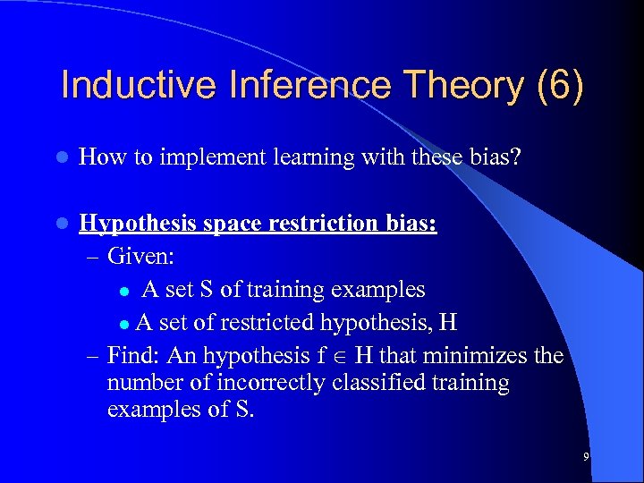Inductive Inference Theory (6) l How to implement learning with these bias? l Hypothesis space restriction bias: – Given: l A set S of training examples l A set of restricted hypothesis, H – Find: An hypothesis f H that minimizes the number of incorrectly classified training examples of S. 9

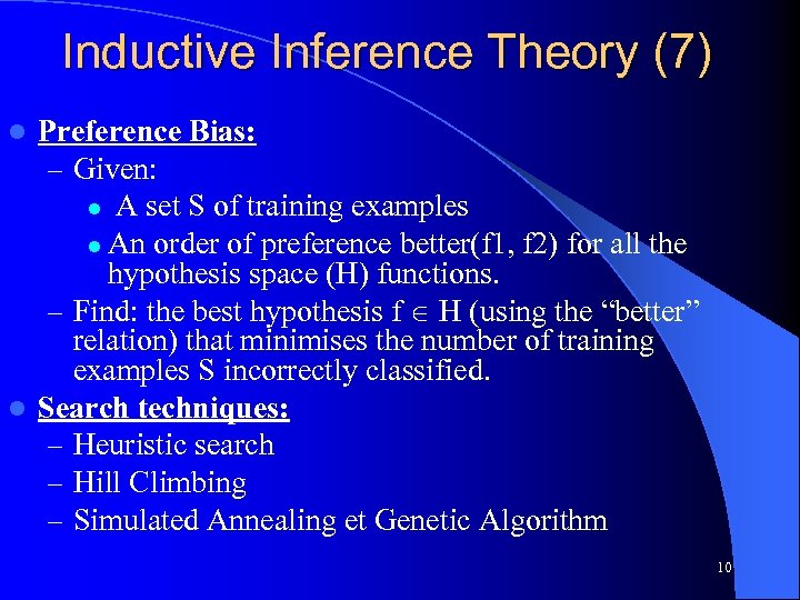Inductive Inference Theory (7) Preference Bias: – Given: l A set S of training examples l An order of preference better(f 1, f 2) for all the hypothesis space (H) functions. – Find: the best hypothesis f H (using the “better” relation) that minimises the number of training examples S incorrectly classified. l Search techniques: – Heuristic search – Hill Climbing – Simulated Annealing et Genetic Algorithm l 10

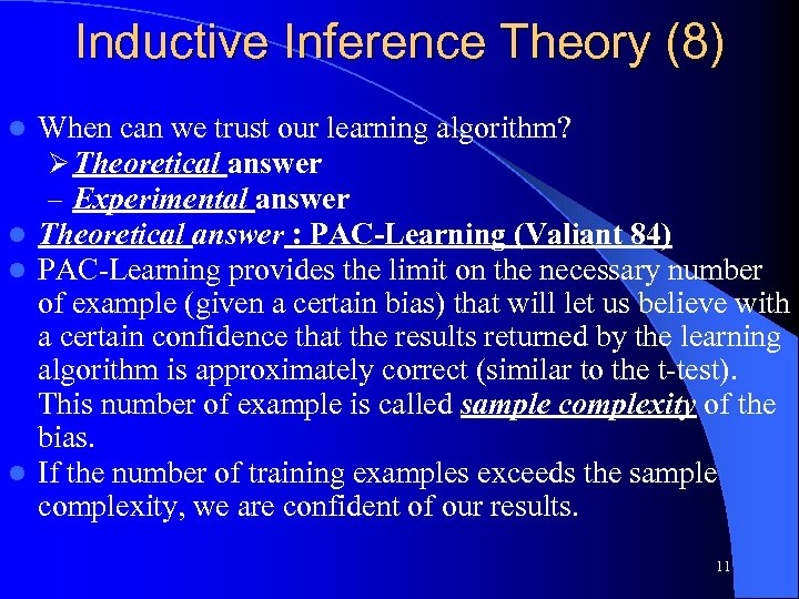Inductive Inference Theory (8) When can we trust our learning algorithm? Ø Theoretical answer – Experimental answer l Theoretical answer : PAC-Learning (Valiant 84) l PAC-Learning provides the limit on the necessary number of example (given a certain bias) that will let us believe with a certain confidence that the results returned by the learning algorithm is approximately correct (similar to the t-test). This number of example is called sample complexity of the bias. l If the number of training examples exceeds the sample complexity, we are confident of our results. l 11

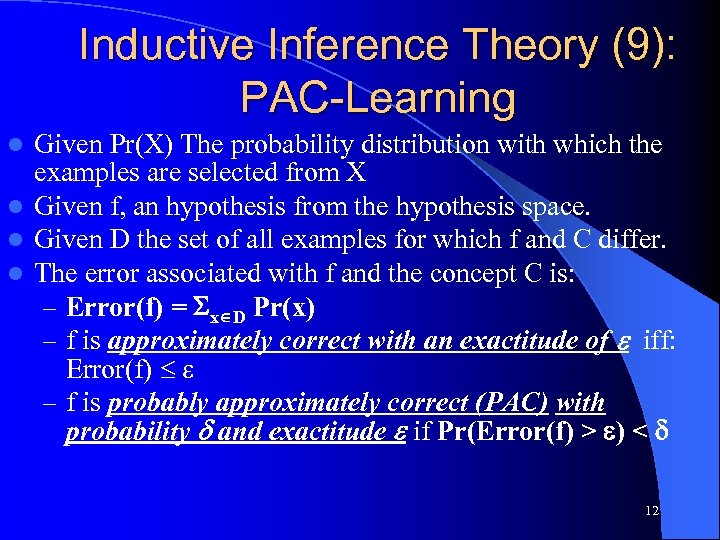Inductive Inference Theory (9): PAC-Learning Given Pr(X) The probability distribution with which the examples are selected from X l Given f, an hypothesis from the hypothesis space. l Given D the set of all examples for which f and C differ. l The error associated with f and the concept C is: – Error(f) = x D Pr(x) – f is approximately correct with an exactitude of iff: Error(f) – f is probably approximately correct (PAC) with probability and exactitude if Pr(Error(f) > ) < l 12

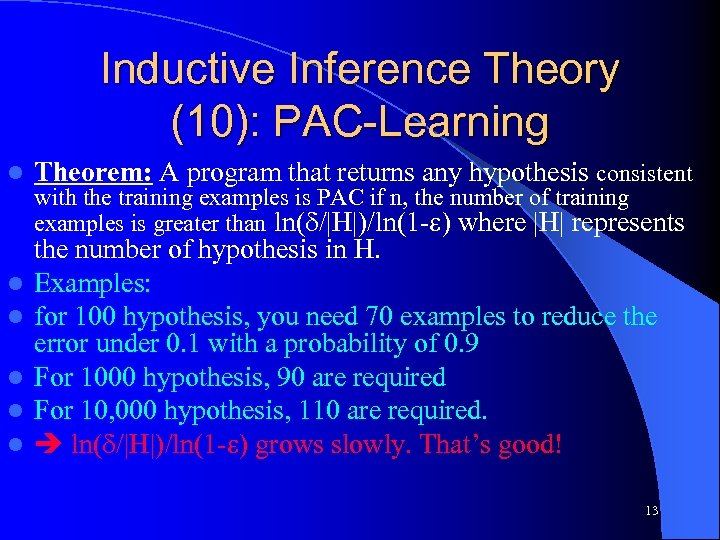Inductive Inference Theory (10): PAC-Learning l l l Theorem: A program that returns any hypothesis consistent with the training examples is PAC if n, the number of training examples is greater than ln( /|H|)/ln(1 - ) where |H| represents the number of hypothesis in H. Examples: for 100 hypothesis, you need 70 examples to reduce the error under 0. 1 with a probability of 0. 9 For 1000 hypothesis, 90 are required For 10, 000 hypothesis, 110 are required. ln( /|H|)/ln(1 - ) grows slowly. That’s good! 13

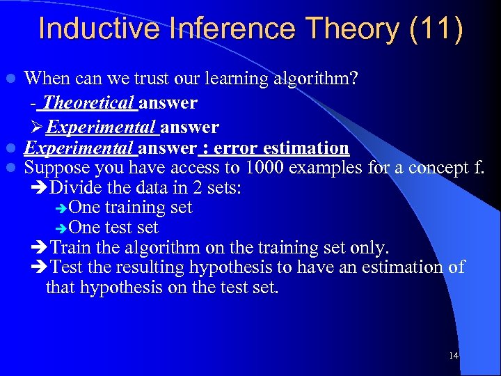Inductive Inference Theory (11) When can we trust our learning algorithm? - Theoretical answer Ø Experimental answer l Experimental answer : error estimation l Suppose you have access to 1000 examples for a concept f. Divide the data in 2 sets: One training set One test set Train the algorithm on the training set only. Test the resulting hypothesis to have an estimation of that hypothesis on the test set. l 14

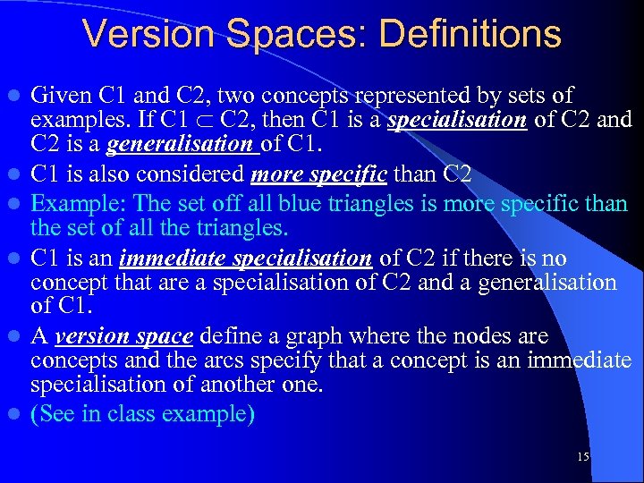Version Spaces: Definitions l l l Given C 1 and C 2, two concepts represented by sets of examples. If C 1 C 2, then C 1 is a specialisation of C 2 and C 2 is a generalisation of C 1 is also considered more specific than C 2 Example: The set off all blue triangles is more specific than the set of all the triangles. C 1 is an immediate specialisation of C 2 if there is no concept that are a specialisation of C 2 and a generalisation of C 1. A version space define a graph where the nodes are concepts and the arcs specify that a concept is an immediate specialisation of another one. (See in class example) 15

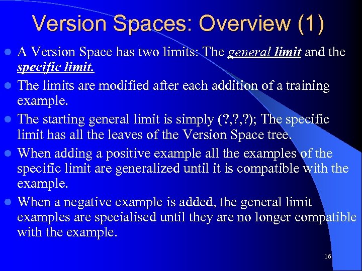Version Spaces: Overview (1) l l l A Version Space has two limits: The general limit and the specific limit. The limits are modified after each addition of a training example. The starting general limit is simply (? , ? ); The specific limit has all the leaves of the Version Space tree. When adding a positive example all the examples of the specific limit are generalized until it is compatible with the example. When a negative example is added, the general limit examples are specialised until they are no longer compatible with the example. 16

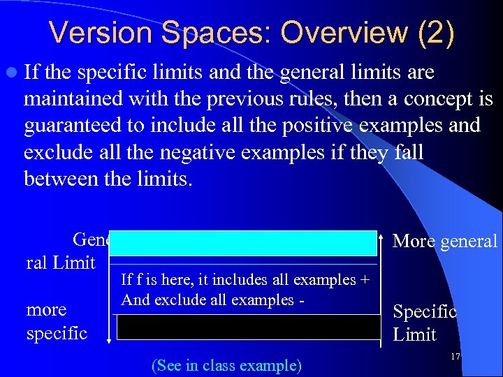Version Spaces: Overview (2) l If the specific limits and the general limits are maintained with the previous rules, then a concept is guaranteed to include all the positive examples and exclude all the negative examples if they fall between the limits. Gene ral Limit more specific More general If f is here, it includes all examples + And exclude all examples - (See in class example) Specific Limit 17

Decision Tree: Introduction The simplest form of learning is the memorization of all the training examples. l Problem: Memorization is not useful for new examples We need to find ways to generalize beyond the training examples. l Possible Solution: Instead of memorizing each attributes of each examples, we can memorize only those that distinguish between positive and negative examples. That is what the decision tree does. l Notice: The same set of example can be represented by different trees. Occam’s Razor tells you to take the smallest tree. (See in class example) l 18

Decision tree: Construction Step 1: We choose an attribute A (= node 0) and split the example by the value of this attribute. Each of these groups correspond to a child of node 0. l Step 2: For each descendant of node 0, if the examples of this descendant are homogenous (have the same class), we stop. l Step 3: If the examples of this descendent are not homogenous, then we call the procedure recursively on that descendent. l (See in class example) 19 l

Decision Tree: Choosing attributes that lead to small trees (I) To obtain a small tree, it is possible to minimize the measure of entropy in the trees that the attribute split generates. l The entropy and information are linked in the following way: The more there is entropy in a set S, the more information is necessary in order to guess correctly an element of this set. l Information: What is the best strategy to guess a number given a finite set S of numbers? What is the smallest number of questions necessary to find the right answer? Answer: Log 2|S| where |S| is the cardinality of S. l 20

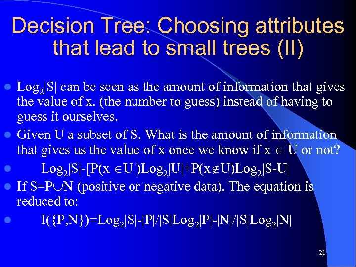Decision Tree: Choosing attributes that lead to small trees (II) l l l Log 2|S| can be seen as the amount of information that gives the value of x. (the number to guess) instead of having to guess it ourselves. Given U a subset of S. What is the amount of information that gives us the value of x once we know if x U or not? Log 2|S|-[P(x U )Log 2|U|+P(x U)Log 2|S-U| If S=P N (positive or negative data). The equation is reduced to: I({P, N})=Log 2|S|-|P|/|S|Log 2|P|-|N|/|S|Log 2|N| 21

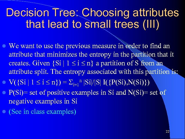Decision Tree: Choosing attributes that lead to small trees (III) We want to use the previous measure in order to find an attribute that minimizes the entropy in the partition that it creates. Given {Si | 1 i n} a partition of S from an attribute split. The entropy associated with this partition is: l V({Si | 1 i n}) = i=1 n |Si|/|S| I({P(Si), N(Si)}) l P(Si)= set of positive examples in Si and N(Si)= set of negative examples in Si l (See in class examples) l 22

Decision Tree: Other questions. l We have to find a way to deal with attributes with continuous values or discrete values with a very large set. l We have to find a way to deal with missing values. l We have to find a way to deal with noise (errors) in the example’s class and in the attribute values. 23

Neural Network: Introduction (I) What is a neural network? l It is a formalism inspired by biological systems and that is composed of units that perform simple mathematical operations in parallel. l Examples of simple mathematical operation units: – Addition unit – Multiplication unit – Threshold (Continous (example: the Sigmoïd) or not) (See in class illustration) l 24

Neural Network: Learning (I) l l l The units are connected in order to create a network capable of computing complicated functions. (See in class example: 2 representations) Since the network has a sigmoid output, it implements a function f(x 1, x 2, x 3, x 4) where the output is in the range [0, 1] We are interested in neural network capable of learning that function. Learning consists of searching in the space of all the matrices of weight values, a combination of weights that satisfy a positive and negative database of the four attributes 25 (x 1, x 2, x 3, x 4) and two class (y=1, y=0)

Neural Network: Learning (II) l Notice that a Neural Network with a set of adjustable weights represent a restricted hypothesis space corresponding to a family of functions. The size of this space can be increased or decreased by changing the number of hidden units in the network. l Learning is done by a hill-climbing approach called backpropagation and is based on the paradigm of search by gradient. 26

Neural Network: Learning (III) l The idea of search by gradient is to take small steps in the direction that minimize the gradient (or derivative) of the error of the function we are trying to learn. l When the gradient is zero we have reached a local minimum that we hope is also the global minimum. l (more details covered in class) 27