CSE 634 Data Mining Techniques Professor Anita Wasilewska

CSE 634 Data Mining Techniques Professor Anita Wasilewska SUNY Stony Brook CLUSTER ANALYSIS By: Arthy Krishnamurthy & Jing Tun Spring 2005

References • Jiawei Han and Michelle Kamber. Data Mining Concept and Techniques (Chapter 8). Morgan Kaufman, 2002. • M. Ester, H. P. Kriegel, J. Sander, and X. Xu. A density-based algorithm for discovering clusters in large spatial databases. KDD'96. http: //ifsc. ualr. edu/xwxu/publications/kdd-96. pdf • K-means and Hierachical Clustering. Statistical data mining tutorial slides by Andrew Moore: http: //www 2. cs. cmu. edu/~awm/tutorials/kmeans. html • How to explain hierarchical clustering. http: //www. analytictech. com/networks/hiclus. htm • Teknomo, Kardi. K-means Clustering Numerical Example. http: //people. revoledu. com/kardi/tutorial/k. Mean/Numerical. E xample. htm

Outline • What is Cluster Analysis? • Applications • Data Types and Distance Metrics • Clustering in Real Databases • Major Clustering Methods • Outlier Analysis • Summary

What is Cluster Analysis? • Cluster: a collection of data objects • Similar to the objects in the same cluster (Intraclass similarity) • Dissimilar to the objects in other clusters (Interclass dissimilarity) • Cluster analysis • Statistical method for grouping a set of data objects into clusters • A good clustering method produces high quality clusters with high intraclass similarity and low interclass similarity • Clustering is unsupervised classification • Can be a stand-alone tool or as a preprocessing step for other algorithms

Outline • What is Cluster Analysis? • Applications • Data Types and Distance Metrics • Clustering in Real Databases • Major Clustering Methods • Outlier Analysis • Summary

Examples of Clustering Applications • Marketing: Help marketers discover distinct groups in their customer bases, and then use this knowledge to develop targeted marketing programs • Insurance: Identifying groups of motor insurance policy holders with a high average claim cost • City-planning: Identifying groups of houses according to their house type, value, and geographical location • Earth-quake studies: Observed earth quake epicenters should be clustered along continent faults

Outline • What is Cluster Analysis? • Applications • Data Types and Distance Metrics • Clustering in Real Databases • Major Clustering Methods • Outlier Analysis • Summary

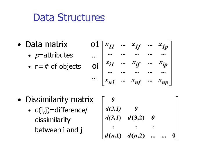Data Structures • Data matrix • p=attributes • n=# of objects o 1 … oi … • Dissimilarity matrix • d(i, j)=difference/ dissimilarity between i and j

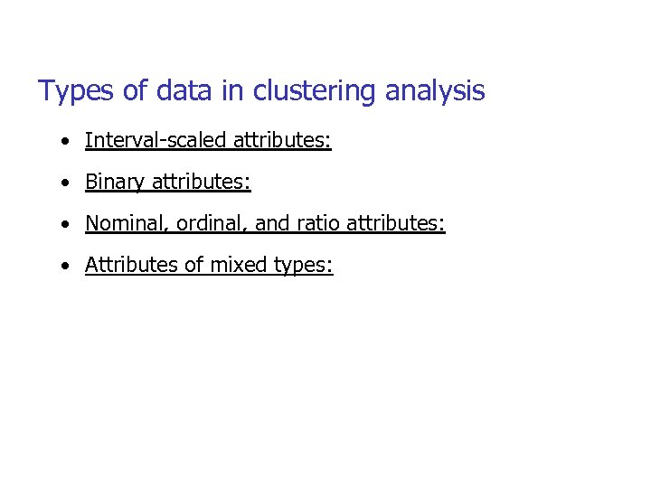Types of data in clustering analysis • Interval-scaled attributes: • Binary attributes: • Nominal, ordinal, and ratio attributes: • Attributes of mixed types:

Interval-scaled attributes • Continuous measurements of a roughly linear scale • E. g. weight, height, temperature, etc. • Standardize data in preprocessing so that all attributes have equal weight • Exceptions: height may be a more important attribute associated with basketball players

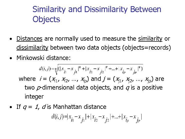Similarity and Dissimilarity Between Objects • Distances are normally used to measure the similarity or dissimilarity between two data objects (objects=records) • Minkowski distance: where i = (xi 1, xi 2, …, xip) and j = (xj 1, xj 2, …, xjp) are two p-dimensional data objects, and q is a positive integer • If q = 1, d is Manhattan distance

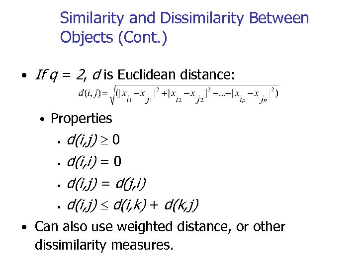Similarity and Dissimilarity Between Objects (Cont. ) • If q = 2, d is Euclidean distance: • Properties • • d(i, j) 0 d(i, i) = 0 d(i, j) = d(j, i) d(i, j) d(i, k) + d(k, j) • Can also use weighted distance, or other dissimilarity measures.

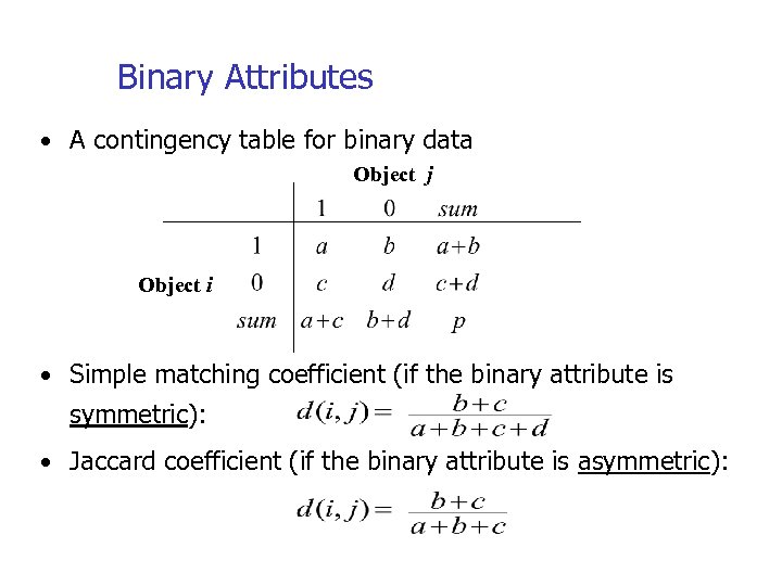Binary Attributes • A contingency table for binary data Object j Object i • Simple matching coefficient (if the binary attribute is symmetric): • Jaccard coefficient (if the binary attribute is asymmetric):

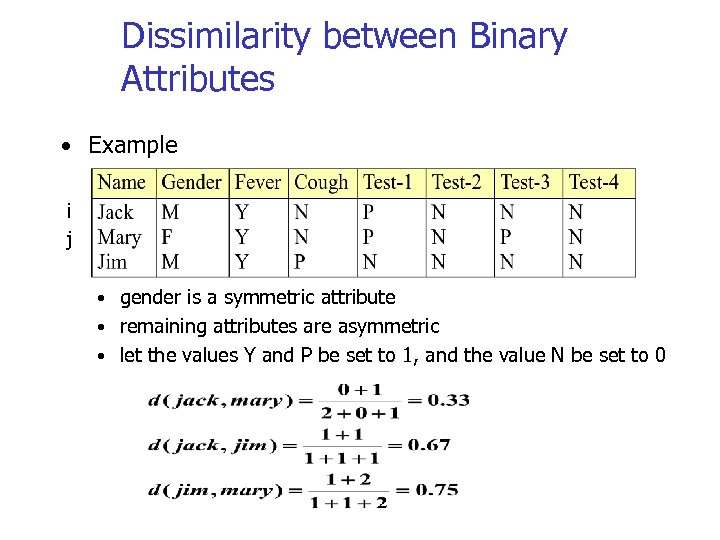Dissimilarity between Binary Attributes • Example i j • gender is a symmetric attribute • remaining attributes are asymmetric • let the values Y and P be set to 1, and the value N be set to 0

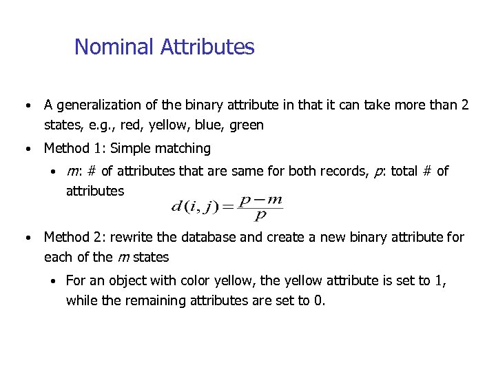Nominal Attributes • A generalization of the binary attribute in that it can take more than 2 states, e. g. , red, yellow, blue, green • Method 1: Simple matching • m: # of attributes that are same for both records, p: total # of attributes • Method 2: rewrite the database and create a new binary attribute for each of the m states • For an object with color yellow, the yellow attribute is set to 1, while the remaining attributes are set to 0.

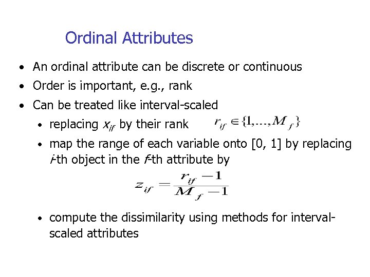Ordinal Attributes • An ordinal attribute can be discrete or continuous • Order is important, e. g. , rank • Can be treated like interval-scaled • replacing xif by their rank • map the range of each variable onto [0, 1] by replacing i-th object in the f-th attribute by • compute the dissimilarity using methods for interval- scaled attributes

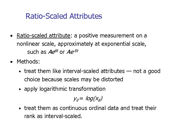Ratio-Scaled Attributes • Ratio-scaled attribute: a positive measurement on a nonlinear scale, approximately at exponential scale, such as Ae. Bt or Ae-Bt • Methods: • treat them like interval-scaled attributes — not a good choice because scales may be distorted • apply logarithmic transformation yif = log(xif) • treat them as continuous ordinal data and treat their rank as interval-scaled.

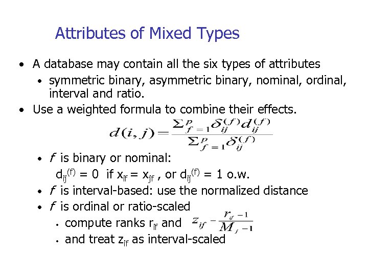Attributes of Mixed Types • A database may contain all the six types of attributes • symmetric binary, asymmetric binary, nominal, ordinal, interval and ratio. • Use a weighted formula to combine their effects. • f is binary or nominal: dij(f) = 0 if xif = xjf , or dij(f) = 1 o. w. • f is interval-based: use the normalized distance • f is ordinal or ratio-scaled • compute ranks rif and • and treat zif as interval-scaled

Outline • What is Cluster Analysis? • Applications • Data Types and Distance Metrics • Clustering in Real Databases • Major Clustering Methods • Outlier Analysis • Summary

Clustering in Real Databases • All data must be transformed into numbers in [0, 1] interval • Weights can be applied • Database attributes can be changed into attributes with binary values • May result in a huge database • Difficulty depending on the type of attribute and the important attributes • Narrow down attributes by their importance

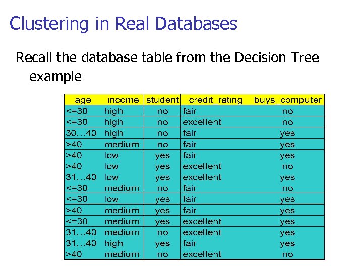Clustering in Real Databases Recall the database table from the Decision Tree example

Outline • What is Cluster Analysis? • Applications • Data Types and Distance Metrics • Clustering in Real Databases • Major Clustering Methods • Outlier Analysis • Summary

Clustering Requirements • Inputs: • Set of attributes • Maximum number of clusters • Number of iterations • Minimum number of elements in any cluster

Major Clustering Approaches • Partitioning algorithms: Divide the set of data objects into various partitions using some criterion • Hierarchy algorithms: Create a hierarchical decomposition of the set of data (or objects) using some criterion • Density-based: based on connectivity and density functions

Partitioning Algorithms: Basic Concept • Partitioning method: Construct a partition of a database D of n objects into a set of k clusters • Input: k • Goal: find a partition of k clusters that optimizes the chosen partitioning criterion[Squared error criterion] • Global optimal: exhaustively enumerate all partitions • Heuristic method: • k-means (Mac. Queen 1967): Each cluster is represented by the center(mean) of the cluster • Variants of the k-means for different data types – k-modes method, etc.

The K-Means Clustering Method • Given k, the k-means algorithm is implemented in 4 steps: • Partition objects into k non-empty subsets • Arbitrarily choose k points as initial centers. • Assign each object to the cluster with the nearest seed point (center). • Calculate the mean of the cluster and update the seed point. • Go back to Step 3, stop when no more new assignment.

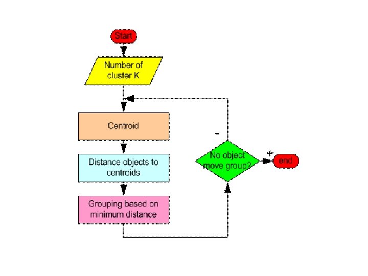
The k-means algorithm: • The basic step of k-means clustering is simple: • Iterate until stable (= no object move group): • Determine the centroid coordinate • Determine the distance of each object to the centroids • Group the object based on minimum distance

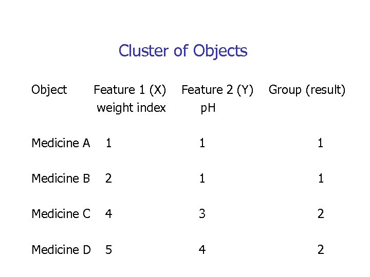
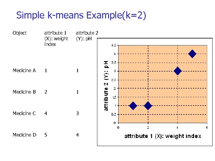Simple k-means Example(k=2) Object attribute 1 (X): weight index attribute 2 (Y): p. H Medicine A 1 1 Medicine B 2 1 Medicine C 4 3 Medicine D 5 4

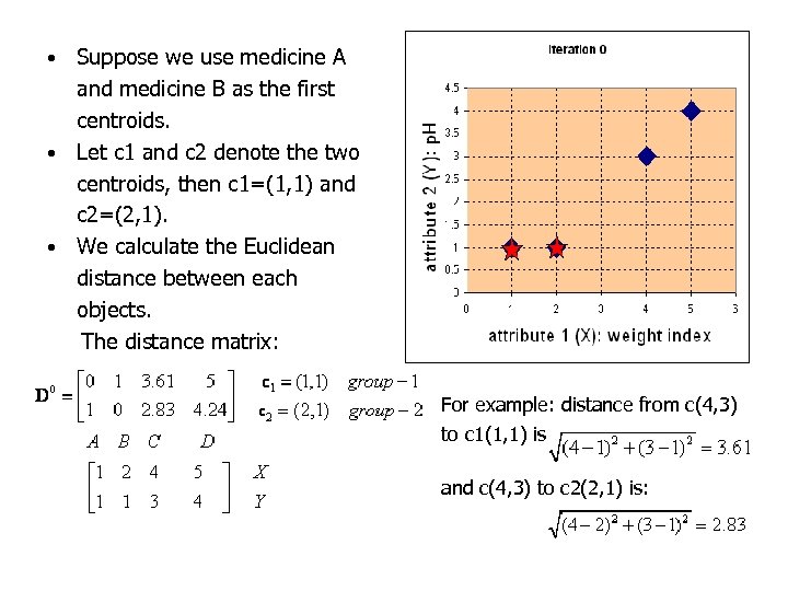Suppose we use medicine A and medicine B as the first centroids. • Let c 1 and c 2 denote the two centroids, then c 1=(1, 1) and c 2=(2, 1). • We calculate the Euclidean distance between each objects. The distance matrix: • For example: distance from c(4, 3) to c 1(1, 1) is and c(4, 3) to c 2(2, 1) is:

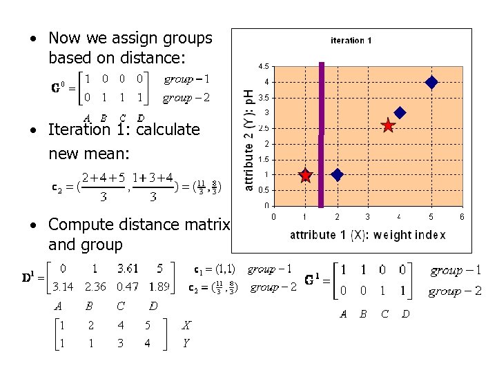• Now we assign groups based on distance: • Iteration 1: calculate new mean: • Compute distance matrix and group

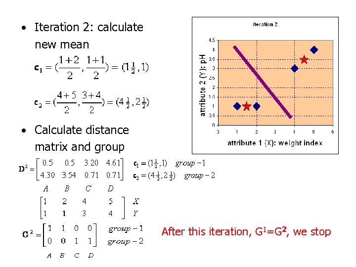• Iteration 2: calculate new mean • Calculate distance matrix and group After this iteration, G 1=G 2, we stop

Cluster of Objects Object Feature 1 (X) weight index Feature 2 (Y) p. H Group (result) Medicine A 1 1 1 Medicine B 2 1 1 Medicine C 4 3 2 Medicine D 5 4 2

Weaknesses of the K-Means Method • Unable to handle noisy data and outliers • Very large or very small values could skew the mean • Not suitable to discover clusters with non-convex shapes

Hierarchical Clustering • Use distance matrix as clustering criteria. This method does not require the number of clusters k as an input, but needs a termination condition. Step 0 a b Step 1 Step 2 Step 3 Step 4 ab abcde c cde d de e Step 4 agglomerative (AGNES) Step 3 Step 2 Step 1 Step 0 divisive (DIANA)

AGNES-Explored • Given a set of N items to be clustered, and an Nx. N distance (or similarity) matrix, the basic process of Johnson's (1967) hierarchical clustering is this: • Start by assigning each item to its own cluster, so that if you have N items, you now have N clusters, each containing just one item. Let the distances (similarities) between the clusters equal the distances (similarities) between the items they contain. • Find the closest (most similar) pair of clusters and merge them into a single cluster, so that now you have one less cluster.

AGNES • Compute distances (similarities) between the new cluster and each of the old clusters. • Repeat steps 2 and 3 until all items are clustered into a single cluster of size N. • Step 3 can be done in different ways, which is what distinguishes single-link from completelink and average-link clustering

Similarity/Distance metrics • single-link clustering, distance = shortest distance • complete-link clustering, distance = longest distance • average-link clustering, distance = average distance from any member of one cluster to any member of the other cluster

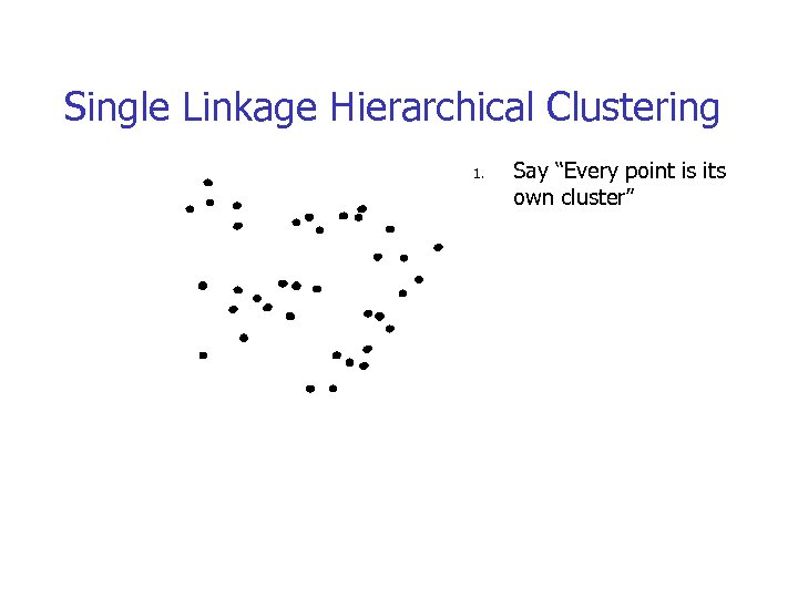Single Linkage Hierarchical Clustering 1. Say “Every point is its own cluster”

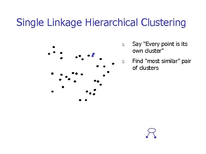Single Linkage Hierarchical Clustering 1. 2. Say “Every point is its own cluster” Find “most similar” pair of clusters

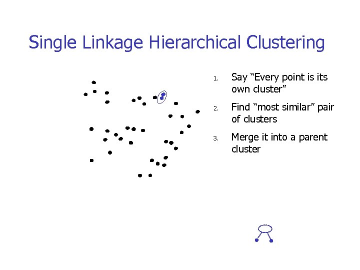Single Linkage Hierarchical Clustering 1. 2. 3. Say “Every point is its own cluster” Find “most similar” pair of clusters Merge it into a parent cluster

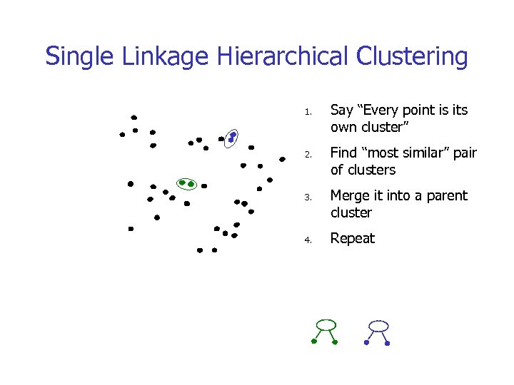Single Linkage Hierarchical Clustering 1. 2. 3. 4. Say “Every point is its own cluster” Find “most similar” pair of clusters Merge it into a parent cluster Repeat

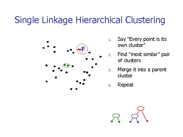Single Linkage Hierarchical Clustering 1. 2. 3. 4. Say “Every point is its own cluster” Find “most similar” pair of clusters Merge it into a parent cluster Repeat

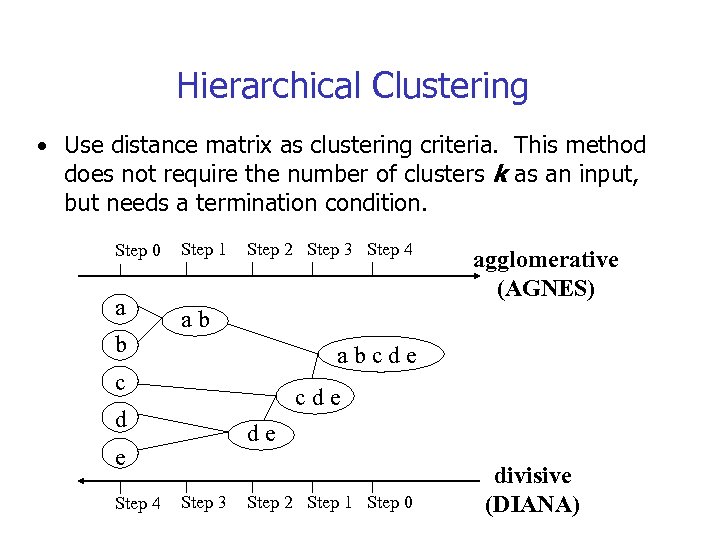
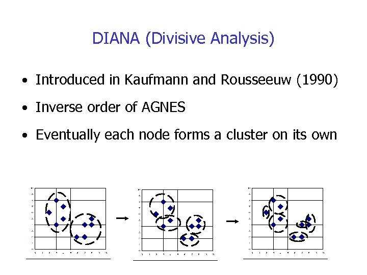DIANA (Divisive Analysis) • Introduced in Kaufmann and Rousseeuw (1990) • Inverse order of AGNES • Eventually each node forms a cluster on its own

Overview • Divisive Clustering starts by placing all objects into a single group. Before we start the procedure, we need to decide on a threshold distance. The procedure is as follows: • The distance between all pairs of objects within the same group is determined and the pair with the largest distance is selected.

Overview-contd • This maximum distance is compared to the threshold distance. • If it is larger than the threshold, this group is divided in two. This is done by placing the selected pair into different groups and using them as seed points. All other objects in this group are examined, and are placed into the new group with the closest seed point. The procedure then returns to Step 1. • If the distance between the selected objects is less than the threshold, the divisive clustering stops. • To run a divisive clustering, you simply need to decide upon a method of measuring the distance between two objects.

Density-Based Clustering Methods • Clustering based on density, such as density-connected points • Cluster = set of “density connected” points. • Major features: • Discover clusters of arbitrary shape • Handle noise • Need “density parameters” as termination condition- (when no new objects can be added to the cluster. ) • Example: • DBSCAN (Ester, et al. 1996) • OPTICS (Ankerst, et al 1999) • DENCLUE (Hinneburg & D. Keim 1998)

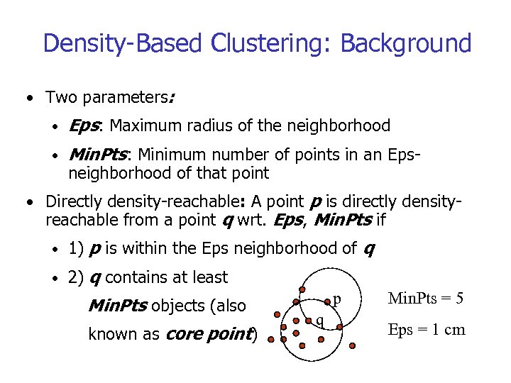Density-Based Clustering: Background • Two parameters: • Eps: Maximum radius of the neighborhood • Min. Pts: Minimum number of points in an Epsneighborhood of that point • Directly density-reachable: A point p is directly density- reachable from a point q wrt. Eps, Min. Pts if • 1) p is within the Eps neighborhood of q • 2) q contains at least Min. Pts objects (also known as core point) p q Min. Pts = 5 Eps = 1 cm

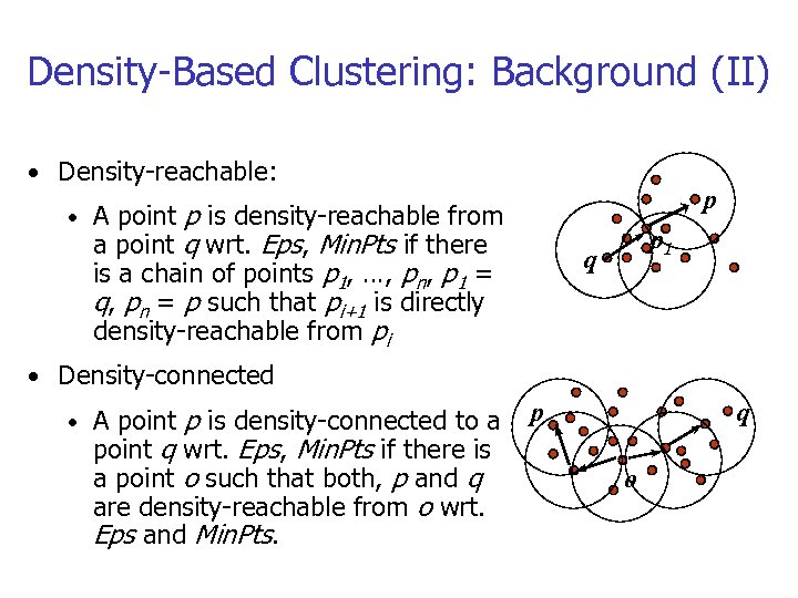Density-Based Clustering: Background (II) • Density-reachable: p p is density-reachable from a point q wrt. Eps, Min. Pts if there is a chain of points p 1, …, pn, p 1 = q, pn = p such that pi+1 is directly density-reachable from pi • A point p 1 q • Density-connected p is density-connected to a point q wrt. Eps, Min. Pts if there is a point o such that both, p and q are density-reachable from o wrt. Eps and Min. Pts. • A point p q o

DBSCAN: The Algorithm • Arbitrary select a point p • Retrieve all points density-reachable from p wrt Eps and Min. Pts. • If p is a core point, a cluster is formed. p is a border point, no points are density-reachable from p and DBSCAN visits the next point of the • If database. • Continue the process until all of the points have been processed.

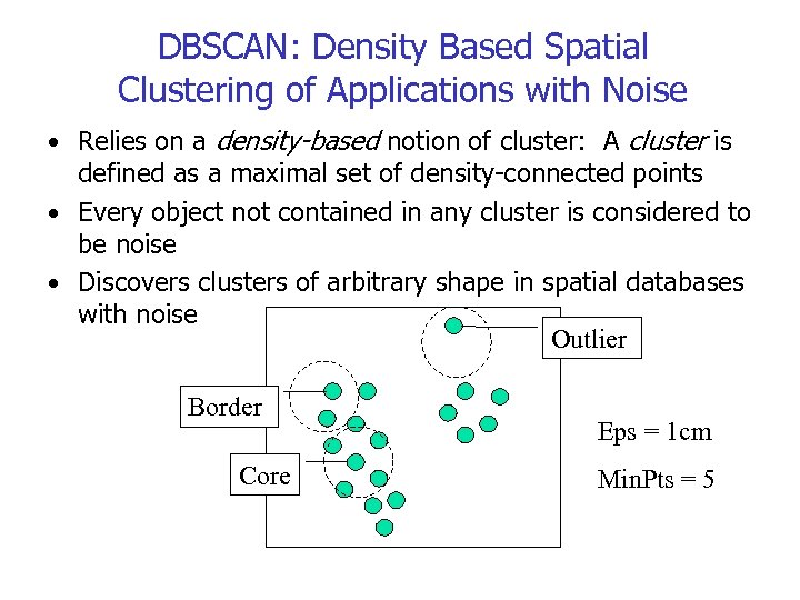DBSCAN: Density Based Spatial Clustering of Applications with Noise • Relies on a density-based notion of cluster: A cluster is defined as a maximal set of density-connected points • Every object not contained in any cluster is considered to be noise • Discovers clusters of arbitrary shape in spatial databases with noise Outlier Border Core Eps = 1 cm Min. Pts = 5

Grid-Based Clustering Method • Quantizes space into a finite number of cells that form a grid structure on which all of the operations for clustering are performed • Example • CLIQUE (CLustering In QUEst) (Agrawal, et al. 1998) • STING (a STatistical INformation Grid approach) (Wang, Yang and Muntz 1997) • Wave. Cluster (Sheikholeslami, Chatterjee, and Zhang 1998)

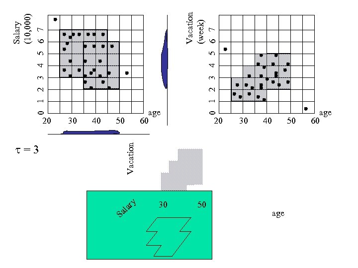
CLIQUE (CLustering In QUEst) • CLIQUE can be considered as both density-based and grid- based • It partitions each dimension into the same number of equal length interval • It partitions an m-dimensional data space into non- overlapping rectangular units • A unit is dense if the fraction of total data points contained in the unit exceeds the input model parameter • A cluster is a maximal set of connected dense units within a subspace

CLIQUE: The Major Steps • Partition the data space and find the number of points that lie inside each cell of the partition. • Identify the subspaces that contain clusters using the Apriori principle • Identify clusters that have the highest density within all of the m dimensions of interest • Generate minimal description for the clusters • Determine maximal regions that cover a cluster of connected dense units for each cluster • Determination of minimal cover for each cluster

30 40 =3 Vacation 20 50 S Salary (10, 000) 0 1 2 3 4 5 6 7 a al ry 30 Vacation (week) 0 1 2 3 4 5 6 7 age 60 20 50 30 40 age 50 age 60

Strength and Weakness of CLIQUE • Strength • It automatically finds subspaces of the highest dimensionality such that high density clusters exist in those subspaces • It is insensitive to the order of records in input and does not presume some canonical data distribution • It scales linearly with the size of input and has good scalability as the number of dimensions in the data increases • Weakness • The accuracy of the clustering result may be degraded at the expense of simplicity of the method

Outline • What is Cluster Analysis? • Applications • Data Types and Distance Metrics • Clustering in Real Databases • Major Clustering Methods • Outlier Analysis • Summary

Outlier Discovery • What are outliers? • The set of objects are considerably dissimilar from the remainder of the data • Example: Sports: Michael Jordon, Wayne Gretzky, . . . • Goal • Given a set of n objects, find the top k objects that are dissimilar, exceptional, or inconsistent with respect to the remaining data • Applications: • Credit card fraud detection • Telecom fraud detection/Cell phone fraud detection.

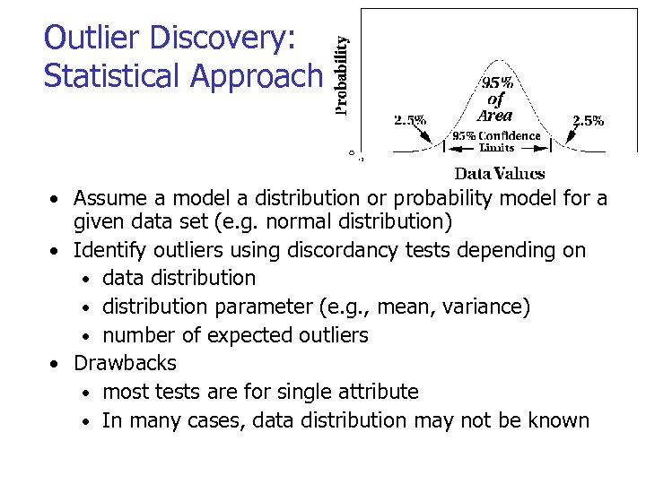Outlier Discovery: Statistical Approaches • Assume a model a distribution or probability model for a given data set (e. g. normal distribution) • Identify outliers using discordancy tests depending on • data distribution • distribution parameter (e. g. , mean, variance) • number of expected outliers • Drawbacks • most tests are for single attribute • In many cases, data distribution may not be known

Outlier Discovery: Distance-Based Approach • Introduced to counter the main limitations imposed by statistical methods • We need multi-dimensional analysis without knowing data distribution. • Distance-based outlier: A DB(p, D)-outlier is an object O in a dataset T such that at least a fraction p of the objects in T lies at a distance greater than D from O

Outlier Discovery: Deviation-Based Approach • Identifies outliers by examining the main characteristics of objects in a group • Objects that “deviate” from this description are considered outliers

Outline • What is Cluster Analysis? • Applications • Data Types and Distance Metrics • Clustering in Real Databases • Major Clustering Methods • Outlier Analysis • Summary

Summary • Cluster analysis groups objects based on their • • • similarity/dissimilarity Clustering is a statistical method therefore preprocessing is necessary if data not in numerical format Clustering is unsupervised learning Clustering algorithms can be categorized into several categories including partitioning methods, hierarchical methods, density-based. Outlier detection and analysis are very useful for fraud detection, etc. and can be performed by statistical, distance-based or deviation-based approaches Clustering has a wide range of applications in the real world.

Thank you !!!