

f5b659dd7365e9b5054c65c1666d3e87.ppt
- Количество слайдов: 105
 CSE 592 Applications of Artificial Intelligence Neural Networks & Data Mining Henry Kautz Winter 2003
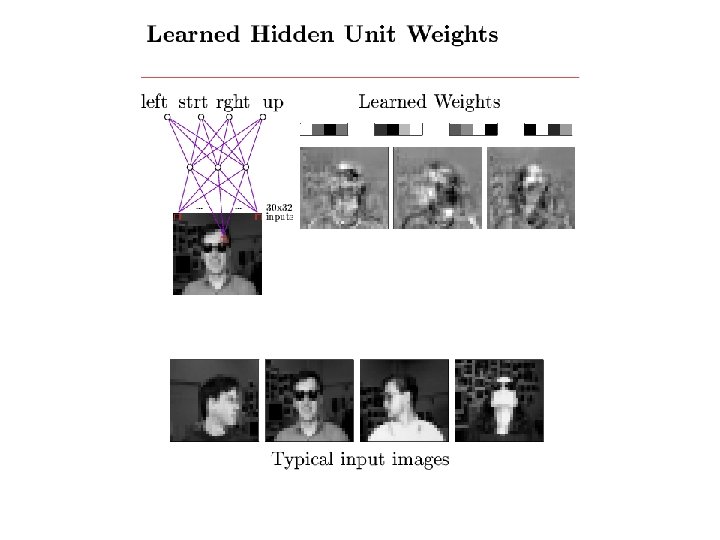
 Kinds of Networks • Feed-forward • Single layer • Multi-layer • Recurrent
 Kinds of Networks • Feed-forward • Single layer • Multi-layer • Recurrent
 Kinds of Networks • Feed-forward • Single layer • Multi-layer • Recurrent
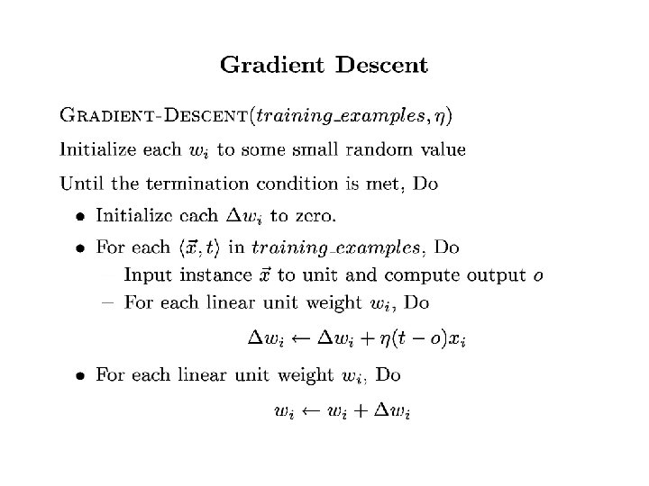
 Basic Idea: Use error between target and actual output to adjust weights
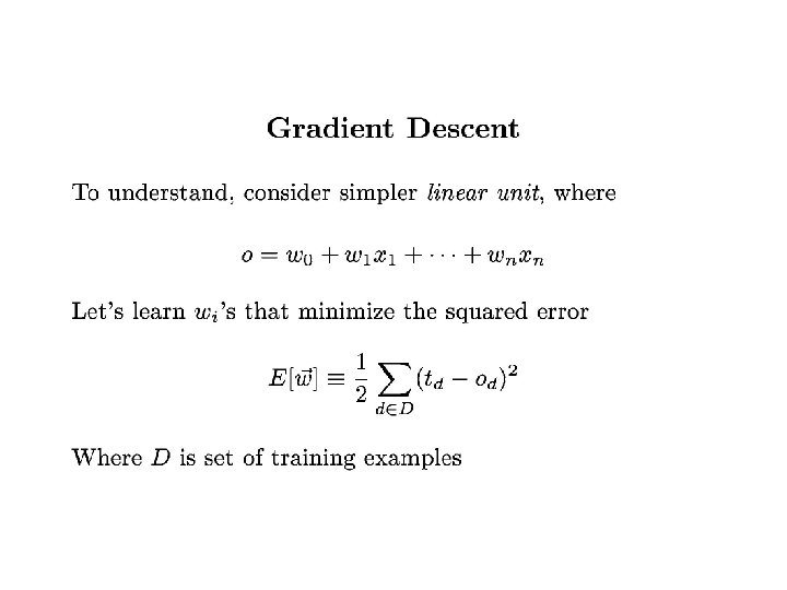
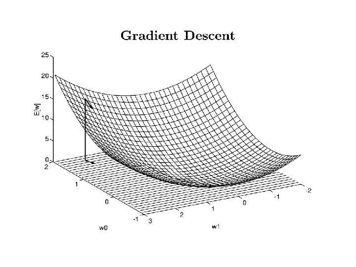
 In other words: take a step the steepest downhill direction
 Multiply by and you get the training rule!
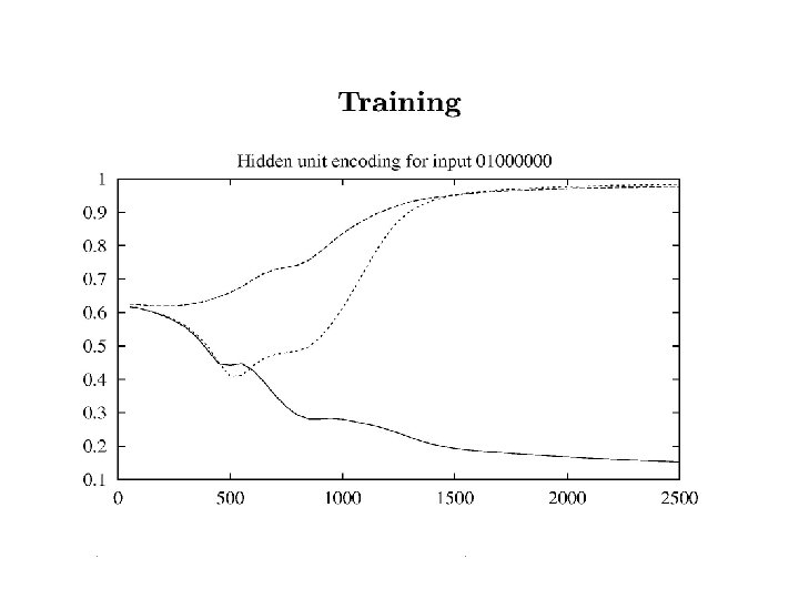
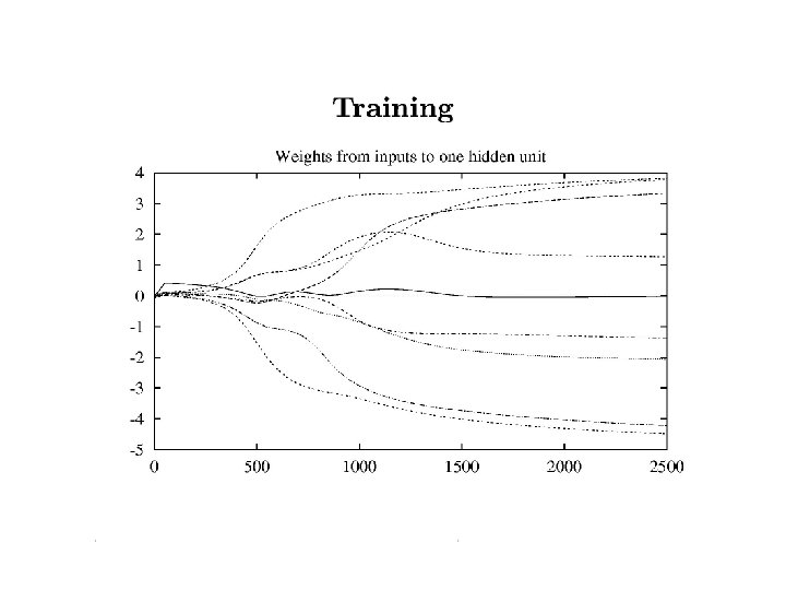
 Demos
Demos
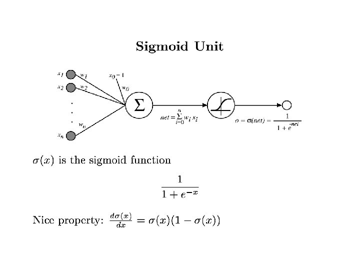
 Deriviative of the sigmoid gives") Training Rule • Single sigmoid unit (a “soft” perceptron) Deriviative of the sigmoid gives this part • Multi-Layered network – Compute values for output units, using observed outputs – For each layer from output back: • Propagate the values back to previous layer • Update incoming weights
Training Rule • Single sigmoid unit (a “soft” perceptron) Deriviative of the sigmoid gives this part • Multi-Layered network – Compute values for output units, using observed outputs – For each layer from output back: • Propagate the values back to previous layer • Update incoming weights
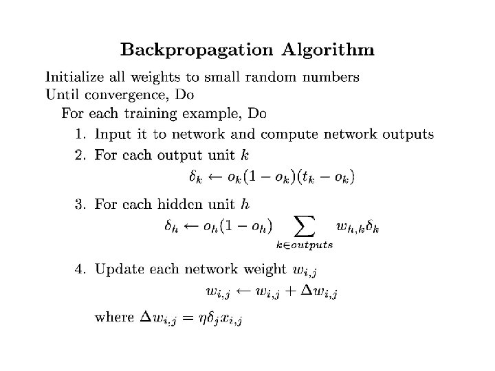
 Derivative of output Weighted error
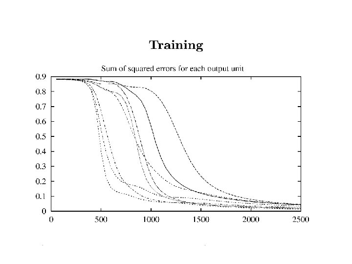
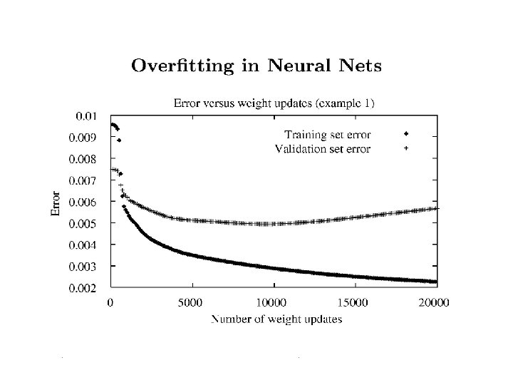
 Be careful not to stop too soon!
 Break!
 Data Mining
 Data Mining n What is the difference between machine learning and data mining?
 Data Mining n What is the difference between machine learning and data mining? n Scale – DM is ML in the large n Focus – DM is more interested in finding “interesting” patterns than in learning to classify data
 Data Mining n What is the difference between machine learning and data mining? n Scale – DM is ML in the large n Focus – DM is more interested in finding “interesting” patterns than in learning to classify data n Marketing!
 Data Mining: Association Rules
 Mining Association Rules in Large Databases n n Introduction to association rule mining Mining single-dimensional Boolean association rules from transactional databases Mining multilevel association rules from transactional databases Mining multidimensional association rules from transactional databases and data warehouse n Constraint-based association mining n Summary
 What Is Association Rule Mining? Association rule mining: n Finding frequent patterns, associations, correlations, or causal structures among sets of items or objects in transaction databases, relational databases, and other information repositories. n Applications: n Basket data analysis, cross-marketing, catalog design, lossleader analysis, clustering, classification, etc. n Examples: n Rule form: “Body ® Head [support, confidence]”. n buys(x, “diapers”) ® buys(x, “beers”) [0. 5%, 60%] n major(x, “CS”) ^ takes(x, “DB”) ® grade(x, “A”) [1%, 75%] n
 database of transactions, (2) each transaction") Association Rules: Basic Concepts n n Given: (1) database of transactions, (2) each transaction is a list of items (purchased by a customer in a visit) Find: all rules that correlate the presence of one set of items with that of another set of items n E. g. , 98% of people who purchase tires and auto accessories also get automotive services done n Applications n n n ? Maintenance Agreement (What the store should do to boost Maintenance Agreement sales) Home Electronics ? (What other products should the store stocks up? ) Attached mailing in direct marketing
Association Rules: Basic Concepts n n Given: (1) database of transactions, (2) each transaction is a list of items (purchased by a customer in a visit) Find: all rules that correlate the presence of one set of items with that of another set of items n E. g. , 98% of people who purchase tires and auto accessories also get automotive services done n Applications n n n ? Maintenance Agreement (What the store should do to boost Maintenance Agreement sales) Home Electronics ? (What other products should the store stocks up? ) Attached mailing in direct marketing
 Association Rules: Definitions n n Set of items: I = {i 1, i 2, …, im} Set of transactions: D = {d 1, d 2, …, dn} Each di I n An association rule: A B where A I, B I, A B = A I B • Means that to some extent A implies B. • Need to measure how strong the implication is.
 Association Rules: Definitions II n The probability of a set A: Where: n k-itemset: tuple of items, or sets of items: Example: {A, B} is a 2 -itemset • The probability of {A, B} is the probability of the set A B, that is the fraction of transactions that contain both A and B. Not the same as P(A B). •
 Association Rules: Definitions III n n Support of a rule A B is the probability of the itemset {A, B}. This gives an idea of how often the rule is relevant. n support(A B ) = P({A, B}) Confidence of a rule A B is the conditional probability of B given A. This gives a measure of how accurate the rule is. n confidence(A B) = P(B|A) = support({A, B}) / support(A)
 Rule Measures: Support and Confidence Customer buys both X: Customer buys beer n Y: Customer buys diaper Find all the rules X Y given thresholds for minimum confidence and minimum support. n support, s, probability that a transaction contains {X, Y} n confidence, c, conditional probability that a transaction having X also contains Y With minimum support 50%, and minimum confidence 50%, we have n A C (50%, 66. 6%) n C A (50%, 100%)
 Association Rule Mining: A Road Map Boolean vs. quantitative associations (Based on the types of values handled) n buys(x, “SQLServer”) ^ buys(x, “DMBook”) ® buys(x, “DBMiner”) [0. 2%, 60%] n age(x, “ 30. . 39”) ^ income(x, “ 42. . 48 K”) ® buys(x, “PC”) [1%, 75%] n Single dimension vs. multiple dimensional associations (see ex. Above) n Single level vs. multiple-level analysis n What brands of beers are associated with what brands of diapers? n Various extensions and analysis n Correlation, causality analysis n n Association does not necessarily imply correlation or causality Maxpatterns and closed itemsets n Constraints enforced n n E. g. , small sales (sum < 100) trigger big buys (sum > 1, 000)?
 Mining Association Rules in Large Databases n n Association rule mining Mining single-dimensional Boolean association rules from transactional databases Mining multilevel association rules from transactional databases Mining multidimensional association rules from transactional databases and data warehouse n From association mining to correlation analysis n Constraint-based association mining n Summary
 Mining Association Rules—An Example Min. support 50% Min. confidence 50% For rule A C: support = support({A, C }) = 50% confidence = support({A, C })/support({A}) = 66. 6% The Apriori principle: Any subset of a frequent itemset must be frequent
 Mining Frequent Itemsets: the Key Step n Find the frequent itemsets: the sets of items that have at least a given minimum support n A subset of a frequent itemset must also be a frequent itemset n n n i. e. , if {A, B} is a frequent itemset, both {A} and {B} should be a frequent itemset Iteratively find frequent itemsets with cardinality from 1 to k (k-itemset) Use the frequent itemsets to generate association rules.
 The Apriori Algorithm n Join Step: Ck is generated by joining Lk-1 with itself Prune Step: Any (k-1)-itemset that is not frequent cannot be n Pseudo-code: n a subset of a frequent k-itemset Ck : Candidate itemset of size k Lk : frequent itemset of size k L 1 = {frequent items} for (k = 1; Lk != ; k++) do begin Ck+1 = candidates generated from Lk for eachtransaction t in database do increment the count of all candidates in Ck+1 that are contained in t Lk+1 = candidates in Ck+1 with min_support end return k Lk;
 The Apriori Algorithm — Example Database D L 1 C 1 Scan D C 2 Scan D L 2 C 3 Scan D L 3
 How to do Generate Candidates? n Suppose the items in Lk-1 are listed in an order n Step 1: self-joining Lk-1 insert into Ck select p. item 1, p. item 2, …, p. itemk-1, q. itemk-1 from Lk-1 p, Lk-1 q where p. item 1=q. item 1, …, p. itemk-2=q. itemk-2, p. itemk-1 < q. itemk-1 n Step 2: pruning forall itemsets c in Ck do forall (k-1)-subsets s of c do if (s is not in Lk-1) then delete from Ck c
 Example of Generating Candidates n L 3={abc, abd, ace, bcd} n Self-joining: L 3*L 3 n n n abcd from abc and abd acde from acd and ace Pruning: n n acde is removed because ade is not in L 3 C 4={abcd}
 Methods to Improve Apriori’s Efficiency n Hash-based itemset counting: A k-itemset whose corresponding hashing bucket count is below the threshold cannot be frequent n Transaction reduction: A transaction that does not contain any frequent k-itemset is useless in subsequent scans n Partitioning: Any itemset that is potentially frequent in DB must be frequent in at least one of the partitions of DB n Sampling: mining on a subset of given data, lower support threshold + a method to determine the completeness n Dynamic itemset counting: add new candidate itemsets only when all of their subsets are estimated to be frequent
 Is Apriori Fast Enough? — Performance Bottlenecks n The core of the Apriori algorithm: n n n Use frequent (k – 1)-itemsets to generate candidate frequent kitemsets Use database scan and pattern matching to collect counts for the candidate itemsets The bottleneck of Apriori: candidate generation n Huge candidate sets: n n n 104 frequent 1 -itemset will generate 107 candidate 2 -itemsets To discover a frequent pattern of size 100, e. g. , {a 1, a 2, …, a 100}, one needs to generate 2100 1030 candidates. Multiple scans of database: n Needs (n +1 ) scans, n is the length of the longest pattern
 Mining Frequent Patterns Without Candidate Generation n Compress a large database into a compact, Frequent. Pattern tree (FP-tree) structure n n n highly condensed, but complete for frequent pattern mining avoid costly database scans Develop an efficient, FP-tree-based frequent pattern mining method n n A divide-and-conquer methodology: decompose mining tasks into smaller ones Avoid candidate generation: sub-database test only!
") Presentation of Association Rules (Table Form )
Presentation of Association Rules (Table Form )
 Visualization of Association Rule Using Plane Graph
 Visualization of Association Rule Using Rule Graph
 Mining Association Rules in Large Databases n n Association rule mining Mining single-dimensional Boolean association rules from transactional databases Mining multilevel association rules from transactional databases Mining multidimensional association rules from transactional databases and data warehouse n From association mining to correlation analysis n Constraint-based association mining n Summary
 Multiple-Level Association Rules Food n n n Items often form hierarchy. bread milk Items at the lower level are expected to have lower 2% wheat white skim support. Rules regarding itemsets at Fraser Sunset appropriate levels could be quite useful. Transaction database can be encoded based on dimensions and levels We can explore shared multilevel mining
 Mining Multi-Level Associations n A top_down, progressive deepening approach: n First find high-level strong rules: milk ® bread [20%, 60%]. n Then find their lower-level “weaker” rules: 2% milk ® wheat bread [6%, 50%]. n Variations at mining multiple-level association rules. n Level-crossed association rules: 2% milk n ® Wonder wheat bread Association rules with multiple, alternative hierarchies: 2% milk ® Wonder bread
 Mining Association Rules in Large Databases n n Association rule mining Mining single-dimensional Boolean association rules from transactional databases Mining multilevel association rules from transactional databases Mining multidimensional association rules from transactional databases and data warehouse n Constraint-based association mining n Summary
 buys(X, “bread”) n Multi-dimensional rules: 2") Multi-Dimensional Association: Concepts n Single-dimensional rules: buys(X, “milk”) buys(X, “bread”) n Multi-dimensional rules: 2 dimensions or predicates n Inter-dimension association rules ( no repeated predicates) age(X, ” 19 -25”) occupation(X, “student”) buys(X, “coke”) n hybrid-dimension association rules (repeated predicates) age(X, ” 19 -25”) buys(X, “popcorn”) buys(X, “coke”) n n Categorical Attributes n finite number of possible values, no ordering among values Quantitative Attributes n numeric, implicit ordering among values
Multi-Dimensional Association: Concepts n Single-dimensional rules: buys(X, “milk”) buys(X, “bread”) n Multi-dimensional rules: 2 dimensions or predicates n Inter-dimension association rules ( no repeated predicates) age(X, ” 19 -25”) occupation(X, “student”) buys(X, “coke”) n hybrid-dimension association rules (repeated predicates) age(X, ” 19 -25”) buys(X, “popcorn”) buys(X, “coke”) n n Categorical Attributes n finite number of possible values, no ordering among values Quantitative Attributes n numeric, implicit ordering among values
 Techniques for Mining MD Associations Search for frequent k-predicate set: n Example: {age, occupation, buys} is a 3 -predicate set. n Techniques can be categorized by how age are treated. 1. Using static discretization of quantitative attributes n Quantitative attributes are statically discretized by using predefined concept hierarchies. 2. Quantitative association rules n Quantitative attributes are dynamically discretized into “bins” based on the distribution of the data. n
 Quantitative Association Rules n n Numeric attributes are dynamically discretized n Such that the confidence or compactness of the rules mined is maximized. 2 -D quantitative association rules: Aquan 1 Aquan 2 Acat Cluster “adjacent” association rules to form general rules using a 2 -D grid. Example: age(X, ” 30 -34”) income(X, ” 24 K - 48 K”) buys(X, ”high resolution TV”)
 Mining Association Rules in Large Databases n n Association rule mining Mining single-dimensional Boolean association rules from transactional databases Mining multilevel association rules from transactional databases Mining multidimensional association rules from transactional databases and data warehouse n Constraint-based association mining n Summary
 Mining Association Rules in Large Databases n n Association rule mining Mining single-dimensional Boolean association rules from transactional databases Mining multilevel association rules from transactional databases Mining multidimensional association rules from transactional databases and data warehouse n Constraint-based association mining n Summary
 Constraint-Based Mining n n Interactive, exploratory mining giga-bytes of data? n Could it be real? — Making good use of constraints! What kinds of constraints can be used in mining? n Knowledge type constraint: classification, association, etc. n Data constraint: SQL-like queries n n Dimension/level constraints: n n in relevance to region, price, brand, customer category. Rule constraints n n Find product pairs sold together in Vancouver in Dec. ’ 98. small sales (price < $10) triggers big sales (sum > $200). Interestingness constraints: n strong rules (min_support 3%, min_confidence 60%).
 Rule Constraints in Association Mining n Two kind of rule constraints: n Rule form constraints: meta-rule guided mining. n n Rule (content) constraint: constraint-based query optimization (Ng, et al. , SIGMOD’ 98). n n P(x, y) ^ Q(x, w) ® takes(x, “database systems”). sum(LHS) < 100 ^ min(LHS) > 20 ^ count(LHS) > 3 ^ sum(RHS) > 1000 1 -variable vs. 2 -variable constraints (Lakshmanan, et al. SIGMOD’ 99): n n 1 -var: A constraint confining only one side (L/R) of the rule, e. g. , as shown above. 2 -var: A constraint confining both sides (L and R). n sum(LHS) < min(RHS) ^ max(RHS) < 5* sum(LHS)
 Constrained Association Query Optimization Problem n Given a CAQ = { (S 1, S 2) | C }, the algorithm should be : sound: It only finds frequent sets that satisfy the given constraints C n complete: All frequent sets satisfy the given constraints C are found A naïve solution: n Apply Apriori for finding all frequent sets, and then to test them for constraint satisfaction one by one. More advanced approach: n Comprehensive analysis of the properties of constraints and try to push them as deeply as possible inside the frequent set computation. n n n
 Summary n n n Association rules offer an efficient way to mine interesting probabilities about data in very large databases. Can be dangerous when misinterpreted as signs of statistically significant causality. The basic Apriori algorithm and it’s extensions allow the user to gather a good deal of information without too many passes through data.
 Data Mining: Clustering
 Preview n Introduction n Partitioning methods n Hierarchical methods n Model-based methods n Density-based methods
 Examples of Clustering Applications n n n Marketing: Help marketers discover distinct groups in their customer bases, and then use this knowledge to develop targeted marketing programs Land use: Identification of areas of similar land use in an earth observation database Insurance: Identifying groups of motor insurance policy holders with a high average claim cost Urban planning: Identifying groups of houses according to their house type, value, and geographical location Seismology: Observed earth quake epicenters should be clustered along continent faults
 What Is a Good Clustering? n A good clustering method will produce clusters with n n n High intra-class similarity Low inter-class similarity Precise definition of clustering quality is difficult n Application-dependent n Ultimately subjective
 Requirements for Clustering in Data Mining n Scalability n Ability to deal with different types of attributes n Discovery of clusters with arbitrary shape n Minimal domain knowledge required to determine input parameters n Ability to deal with noise and outliers n Insensitivity to order of input records n Robustness wrt high dimensionality n Incorporation of user-specified constraints n Interpretability and usability
: d(i, j)") Similarity and Dissimilarity Between Objects n Properties of a metric d(i, j): d(i, j) 0 n d(i, i) = 0 n d(i, j) = d(j, i) n d(i, j) d(i, k) + d(k, j) n
Similarity and Dissimilarity Between Objects n Properties of a metric d(i, j): d(i, j) 0 n d(i, i) = 0 n d(i, j) = d(j, i) n d(i, j) d(i, k) + d(k, j) n
 Major Clustering Approaches n Partitioning: Construct various partitions and then evaluate them by some criterion n Hierarchical: Create a hierarchical decomposition of the set of objects using some criterion n Model-based: Hypothesize a model for each cluster and find best fit of models to data n Density-based: Guided by connectivity and density functions
 Partitioning Algorithms n n Partitioning method: Construct a partition of a database D of n objects into a set of k clusters Given a k, find a partition of k clusters that optimizes the chosen partitioning criterion n Global optimal: exhaustively enumerate all partitions n Heuristic methods: k-means and k-medoids algorithms n k-means (Mac. Queen, 1967): Each cluster is represented by the center of the cluster n k-medoids or PAM (Partition around medoids) (Kaufman & Rousseeuw, 1987): Each cluster is represented by one of the objects in the cluster
 K-Means Clustering n Given k, the k-means algorithm consists of four steps: n Select initial centroids at random. n Assign each object to the cluster with the nearest centroid. n Compute each centroid as the mean of the objects assigned to it. n Repeat previous 2 steps until no change.
 n Example") K-Means Clustering (contd. ) n Example
K-Means Clustering (contd. ) n Example
 n Example") K-Means Clustering (contd. ) n Example
K-Means Clustering (contd. ) n Example
 n Example") K-Means Clustering (contd. ) n Example
K-Means Clustering (contd. ) n Example
 n Example") K-Means Clustering (contd. ) n Example
K-Means Clustering (contd. ) n Example
 n Example") K-Means Clustering (contd. ) n Example
K-Means Clustering (contd. ) n Example
, where") Comments on the K-Means Method n Strengths n n n Relatively efficient: O(tkn), where n is # objects, k is # clusters, and t is # iterations. Normally, k, t << n. Often terminates at a local optimum. The global optimum may be found using techniques such as simulated annealing and genetic algorithms Weaknesses n Applicable only when mean is defined (what about categorical data? ) n Need to specify k, the number of clusters, in advance n Trouble with noisy data and outliers n Not suitable to discover clusters with non-convex shapes
Comments on the K-Means Method n Strengths n n n Relatively efficient: O(tkn), where n is # objects, k is # clusters, and t is # iterations. Normally, k, t << n. Often terminates at a local optimum. The global optimum may be found using techniques such as simulated annealing and genetic algorithms Weaknesses n Applicable only when mean is defined (what about categorical data? ) n Need to specify k, the number of clusters, in advance n Trouble with noisy data and outliers n Not suitable to discover clusters with non-convex shapes
 Hierarchical Clustering n Use distance matrix as clustering criteria. This method does not require the number of clusters k as an input, but needs a termination condition Step 0 a b Step 1 Step 2 Step 3 Step 4 a b c d e c c d e d d e e Step 4 agglomerative (AGNES) Step 3 Step 2 Step 1 Step 0 divisive (DIANA)
 n Produces tree of clusters (nodes) n Initially: each object is") AGNES (Agglomerative Nesting) n Produces tree of clusters (nodes) n Initially: each object is a cluster (leaf) n Recursively merges nodes that have the least dissimilarity n Criteria: min distance, max distance, avg distance, center distance n Eventually all nodes belong to the same cluster (root)
AGNES (Agglomerative Nesting) n Produces tree of clusters (nodes) n Initially: each object is a cluster (leaf) n Recursively merges nodes that have the least dissimilarity n Criteria: min distance, max distance, avg distance, center distance n Eventually all nodes belong to the same cluster (root)
 n Inverse order of AGNES n Start with root cluster containing") DIANA (Divisive Analysis) n Inverse order of AGNES n Start with root cluster containing all objects n Recursively divide into subclusters n Eventually each cluster contains a single object
DIANA (Divisive Analysis) n Inverse order of AGNES n Start with root cluster containing all objects n Recursively divide into subclusters n Eventually each cluster contains a single object
 Other Hierarchical Clustering Methods n n Major weakness of agglomerative clustering methods 2 n Do not scale well: time complexity of at least O(n ), where n is the number of total objects n Can never undo what was done previously Integration of hierarchical with distance-based clustering n BIRCH: uses CF-tree and incrementally adjusts the quality of sub-clusters n CURE: selects well-scattered points from the cluster and then shrinks them towards the center of the cluster by a specified fraction
 Model-Based Clustering n n n Basic idea: Clustering as probability estimation One model for each cluster Generative model: n Probability of selecting a cluster n Probability of generating an object in cluster Find max. likelihood or MAP model Missing information: Cluster membership n Use EM algorithm Quality of clustering: Likelihood of test objects
 http: //ic. arc. nasa. gov/ic/projects/bayes-group/autoclass/ Auto. Class An unsupervised Bayesian classification system that seeks a maximum posterior probability classification. Key features: n determines the number of classes automatically; n can use mixed discrete and real valued data; n can handle missing values – uses EM (Expectation Maximization) n processing time is roughly linear in the amount of the data; n cases have probabilistic class membership; n allows correlation between attributes within a class; n generates reports describing the classes found; and n predicts "test" case class memberships from a "training" classification
 From subtle differences between their infrared spectra, two subgroups of stars were distinguished, where previously no difference was suspected. The difference is confirmed by looking at their positions on this map of the galaxy.
 Clustering: Summary n Introduction n Partitioning methods n Hierarchical methods n Model-based methods
 n n n Next week: Making Decisions n From utility theory to reinforcement learning Finish assignments! Start (or keep rolling on project) – n Today’s status report in my mail ASAP (next week at the latest)