590c83f884dd90d96c954453ec4c7cc0.ppt
- Количество слайдов: 113
 CSE 567 M Computer Systems Analysis © 2006 Raj Jain www. rajjain. com 1 -1
 Text Book q R. Jain, “Art of Computer Systems Performance Analysis, ” Wiley, 1991, ISBN: 0471503363 (Winner of the “ 1992 Best Computer Systems Book” Award from Computer Press Association”) © 2006 Raj Jain www. rajjain. com 1 -2
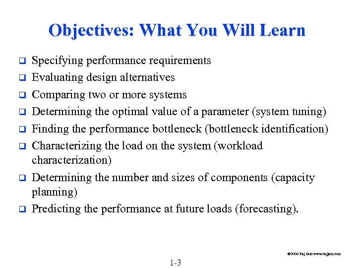 Objectives: What You Will Learn q q q q Specifying performance requirements Evaluating design alternatives Comparing two or more systems Determining the optimal value of a parameter (system tuning) Finding the performance bottleneck (bottleneck identification) Characterizing the load on the system (workload characterization) Determining the number and sizes of components (capacity planning) Predicting the performance at future loads (forecasting). © 2006 Raj Jain www. rajjain. com 1 -3
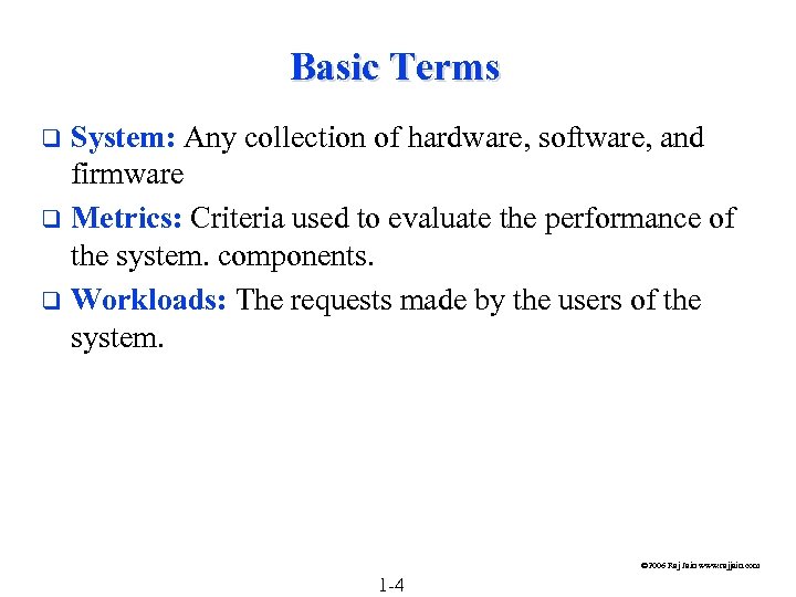 Basic Terms System: Any collection of hardware, software, and firmware q Metrics: Criteria used to evaluate the performance of the system. components. q Workloads: The requests made by the users of the system. q © 2006 Raj Jain www. rajjain. com 1 -4
 Main Parts of the Course An Overview of Performance Evaluation q Measurement Techniques and Tools q Experimental Design and Analysis q © 2006 Raj Jain www. rajjain. com 1 -5
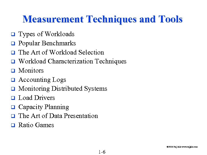 Measurement Techniques and Tools q q q Types of Workloads Popular Benchmarks The Art of Workload Selection Workload Characterization Techniques Monitors Accounting Logs Monitoring Distributed Systems Load Drivers Capacity Planning The Art of Data Presentation Ratio Games © 2006 Raj Jain www. rajjain. com 1 -6
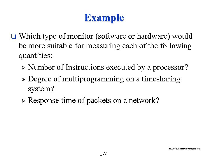 Example q Which type of monitor (software or hardware) would be more suitable for measuring each of the following quantities: Ø Number of Instructions executed by a processor? Ø Degree of multiprogramming on a timesharing system? Ø Response time of packets on a network? © 2006 Raj Jain www. rajjain. com 1 -7
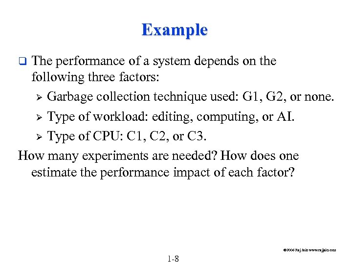 Example The performance of a system depends on the following three factors: Ø Garbage collection technique used: G 1, G 2, or none. Ø Type of workload: editing, computing, or AI. Ø Type of CPU: C 1, C 2, or C 3. How many experiments are needed? How does one estimate the performance impact of each factor? q © 2006 Raj Jain www. rajjain. com 1 -8
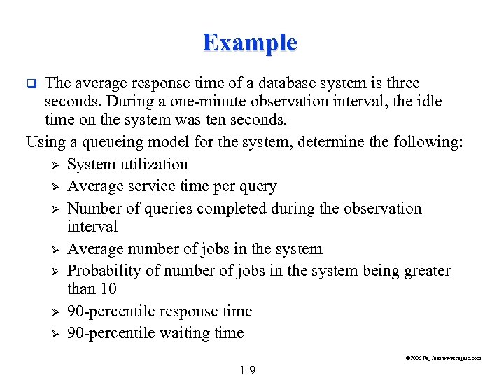 Example The average response time of a database system is three seconds. During a one-minute observation interval, the idle time on the system was ten seconds. Using a queueing model for the system, determine the following: Ø System utilization Ø Average service time per query Ø Number of queries completed during the observation interval Ø Average number of jobs in the system Ø Probability of number of jobs in the system being greater than 10 Ø 90 -percentile response time Ø 90 -percentile waiting time q © 2006 Raj Jain www. rajjain. com 1 -9
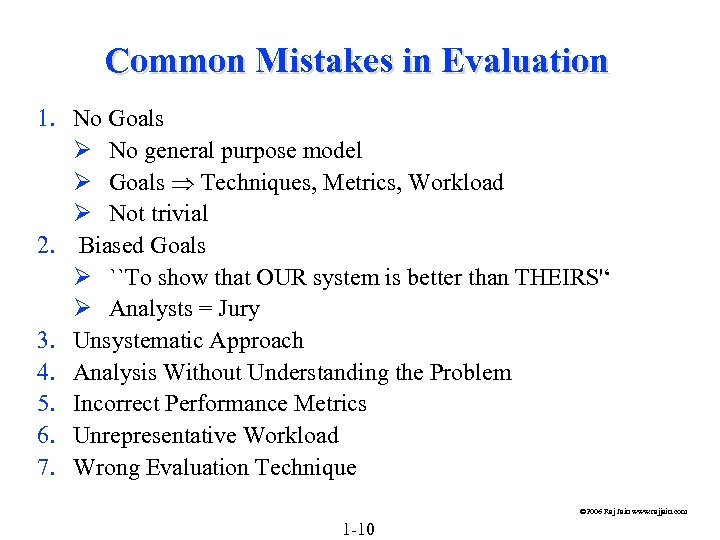 Common Mistakes in Evaluation 1. No Goals Ø No general purpose model Ø Goals Techniques, Metrics, Workload Ø Not trivial 2. Biased Goals Ø ``To show that OUR system is better than THEIRS'‘ Ø Analysts = Jury 3. Unsystematic Approach 4. Analysis Without Understanding the Problem 5. Incorrect Performance Metrics 6. Unrepresentative Workload 7. Wrong Evaluation Technique © 2006 Raj Jain www. rajjain. com 1 -10
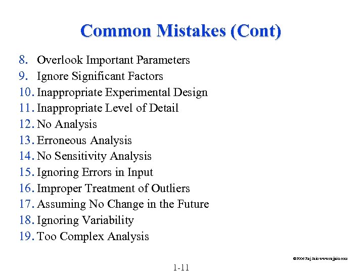 Common Mistakes (Cont) 8. Overlook Important Parameters 9. Ignore Significant Factors 10. Inappropriate Experimental Design 11. Inappropriate Level of Detail 12. No Analysis 13. Erroneous Analysis 14. No Sensitivity Analysis 15. Ignoring Errors in Input 16. Improper Treatment of Outliers 17. Assuming No Change in the Future 18. Ignoring Variability 19. Too Complex Analysis © 2006 Raj Jain www. rajjain. com 1 -11
 Common Mistakes (Cont) 20. Improper Presentation of Results 21. Ignoring Social Aspects 22. Omitting Assumptions and Limitations © 2006 Raj Jain www. rajjain. com 1 -12
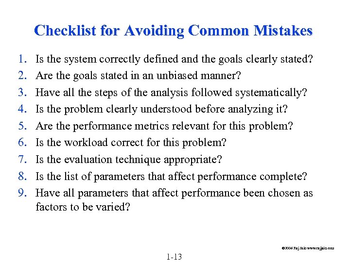 Checklist for Avoiding Common Mistakes 1. 2. 3. 4. 5. 6. 7. 8. 9. Is the system correctly defined and the goals clearly stated? Are the goals stated in an unbiased manner? Have all the steps of the analysis followed systematically? Is the problem clearly understood before analyzing it? Are the performance metrics relevant for this problem? Is the workload correct for this problem? Is the evaluation technique appropriate? Is the list of parameters that affect performance complete? Have all parameters that affect performance been chosen as factors to be varied? © 2006 Raj Jain www. rajjain. com 1 -13
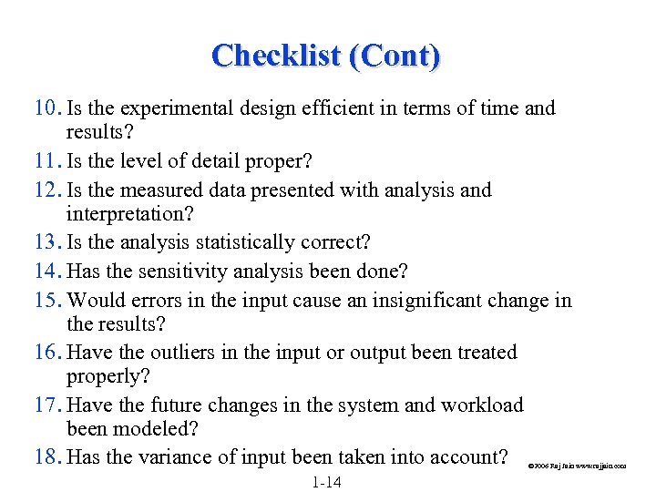 Checklist (Cont) 10. Is the experimental design efficient in terms of time and results? 11. Is the level of detail proper? 12. Is the measured data presented with analysis and interpretation? 13. Is the analysis statistically correct? 14. Has the sensitivity analysis been done? 15. Would errors in the input cause an insignificant change in the results? 16. Have the outliers in the input or output been treated properly? 17. Have the future changes in the system and workload been modeled? 18. Has the variance of input been taken into account? © 2006 Raj Jain www. rajjain. com 1 -14
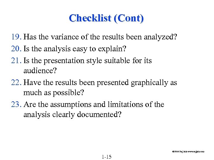 Checklist (Cont) 19. Has the variance of the results been analyzed? 20. Is the analysis easy to explain? 21. Is the presentation style suitable for its audience? 22. Have the results been presented graphically as much as possible? 23. Are the assumptions and limitations of the analysis clearly documented? © 2006 Raj Jain www. rajjain. com 1 -15
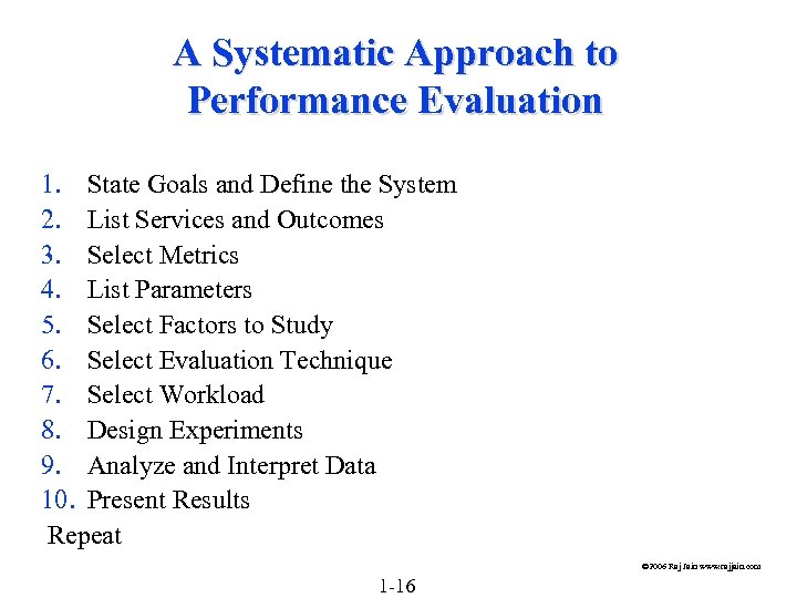 A Systematic Approach to Performance Evaluation 1. State Goals and Define the System 2. List Services and Outcomes 3. Select Metrics 4. List Parameters 5. Select Factors to Study 6. Select Evaluation Technique 7. Select Workload 8. Design Experiments 9. Analyze and Interpret Data 10. Present Results Repeat © 2006 Raj Jain www. rajjain. com 1 -16
 Criteria for Selecting an Evaluation Technique © 2006 Raj Jain www. rajjain. com 1 -17
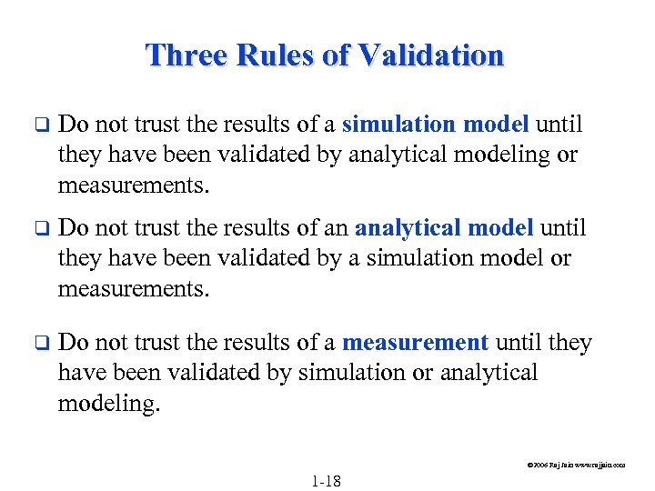 Three Rules of Validation q Do not trust the results of a simulation model until they have been validated by analytical modeling or measurements. q Do not trust the results of an analytical model until they have been validated by a simulation model or measurements. q Do not trust the results of a measurement until they have been validated by simulation or analytical modeling. © 2006 Raj Jain www. rajjain. com 1 -18
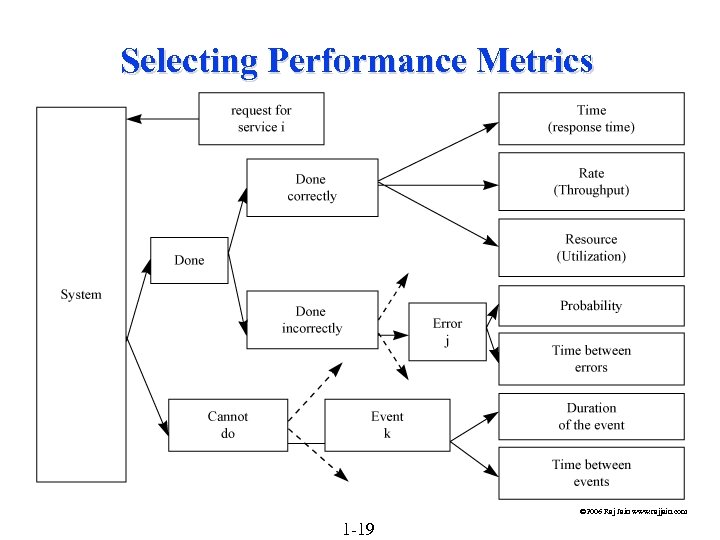 Selecting Performance Metrics © 2006 Raj Jain www. rajjain. com 1 -19
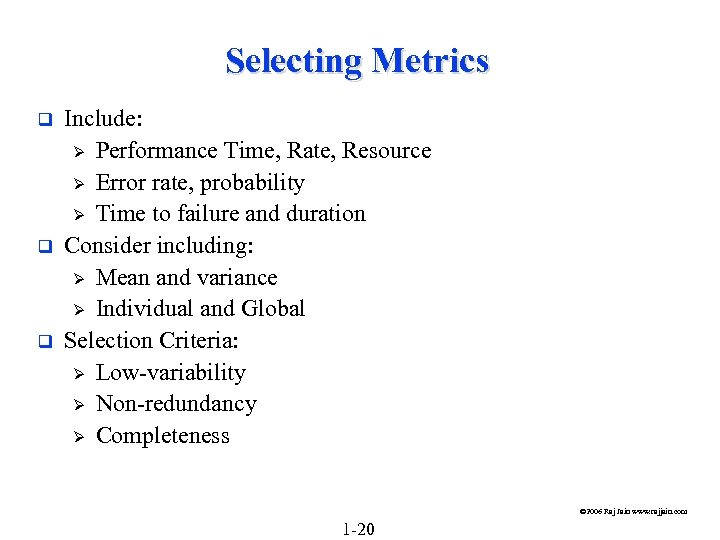 Selecting Metrics q q q Include: Ø Performance Time, Rate, Resource Ø Error rate, probability Ø Time to failure and duration Consider including: Ø Mean and variance Ø Individual and Global Selection Criteria: Ø Low-variability Ø Non-redundancy Ø Completeness © 2006 Raj Jain www. rajjain. com 1 -20
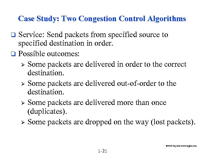 Case Study: Two Congestion Control Algorithms Service: Send packets from specified source to specified destination in order. q Possible outcomes: Ø Some packets are delivered in order to the correct destination. Ø Some packets are delivered out-of-order to the destination. Ø Some packets are delivered more than once (duplicates). Ø Some packets are dropped on the way (lost packets). q © 2006 Raj Jain www. rajjain. com 1 -21
 Case Study (Cont) q Performance: For packets delivered in order, Ø Time-rate-resource q Response time to deliver the packets q Throughput: the number of packets per unit of time. q Processor time per packet on the source end system. q Processor time per packet on the destination end systems. q Processor time per packet on the intermediate systems. Ø Variability of the response time Retransmissions q Response time: the delay inside the network © 2006 Raj Jain www. rajjain. com 1 -22
 Case Study (Cont) Out-of-order packets consume buffers Probability of out-of-order arrivals. Ø Duplicate packets consume the network resources Probability of duplicate packets Ø Lost packets require retransmission Probability of lost packets Ø Too much loss cause disconnection Probability of disconnect Ø © 2006 Raj Jain www. rajjain. com 1 -23
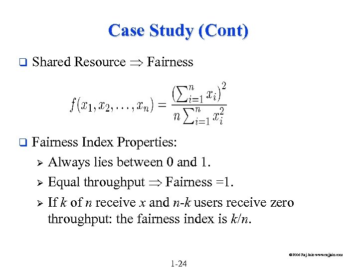 Case Study (Cont) q Shared Resource Fairness q Fairness Index Properties: Ø Always lies between 0 and 1. Ø Equal throughput Fairness =1. Ø If k of n receive x and n-k users receive zero throughput: the fairness index is k/n. © 2006 Raj Jain www. rajjain. com 1 -24
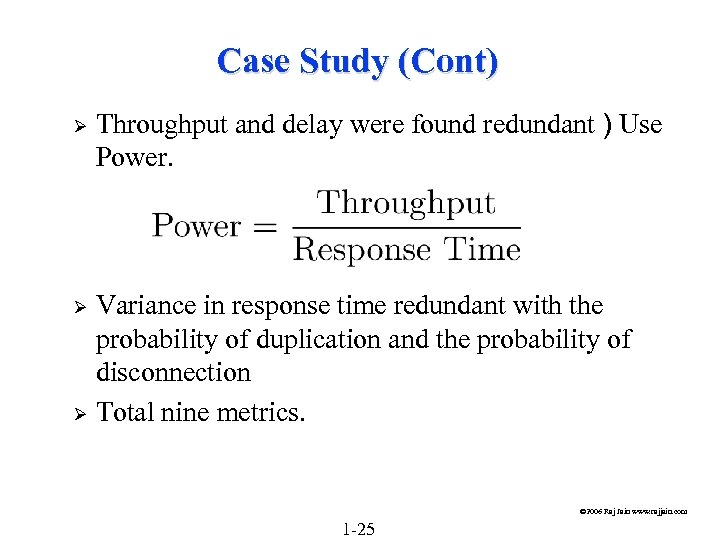 Case Study (Cont) Ø Throughput and delay were found redundant ) Use Power. Variance in response time redundant with the probability of duplication and the probability of disconnection Ø Total nine metrics. Ø © 2006 Raj Jain www. rajjain. com 1 -25
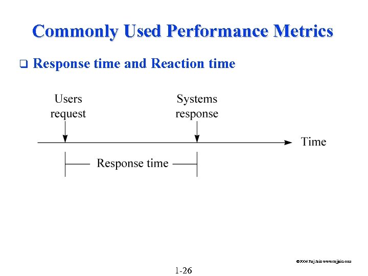 Commonly Used Performance Metrics q Response time and Reaction time © 2006 Raj Jain www. rajjain. com 1 -26
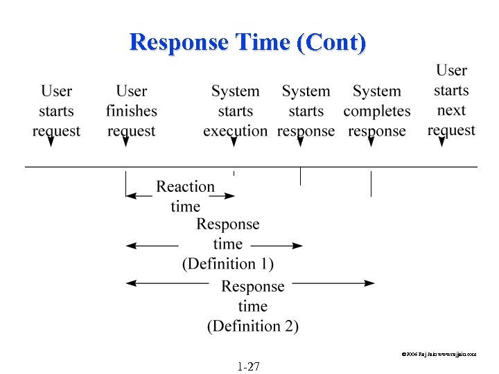 Response Time (Cont) © 2006 Raj Jain www. rajjain. com 1 -27
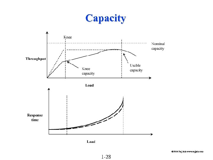 Capacity © 2006 Raj Jain www. rajjain. com 1 -28
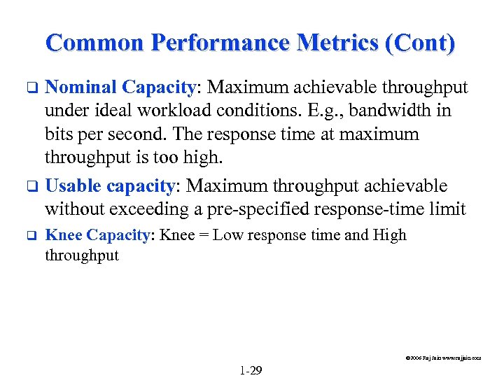 Common Performance Metrics (Cont) Nominal Capacity: Maximum achievable throughput under ideal workload conditions. E. g. , bandwidth in bits per second. The response time at maximum throughput is too high. q Usable capacity: Maximum throughput achievable without exceeding a pre-specified response-time limit q q Knee Capacity: Knee = Low response time and High throughput © 2006 Raj Jain www. rajjain. com 1 -29
 Common Performance Metrics (cont) q q q Turnaround time = the time between the submission of a batch job and the completion of its output. Stretch Factor: The ratio of the response time with multiprogramming to that without multiprogramming. Throughput: Rate (requests per unit of time) Examples: Ø Jobs per second Ø Requests per second Ø Millions of Instructions Per Second (MIPS) Ø Millions of Floating Point Operations Per Second (MFLOPS) Ø Packets Per Second (PPS) Ø Bits per second (bps) Ø Transactions Per Second (TPS) © 2006 Raj Jain www. rajjain. com 1 -30
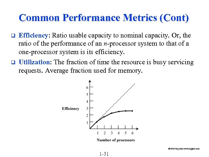 Common Performance Metrics (Cont) q q Efficiency: Ratio usable capacity to nominal capacity. Or, the ratio of the performance of an n-processor system to that of a one-processor system is its efficiency. Utilization: The fraction of time the resource is busy servicing requests. Average fraction used for memory. © 2006 Raj Jain www. rajjain. com 1 -31
 Common Performance Metrics (Cont) Reliability: Ø Probability of errors Ø Mean time between errors (error-free seconds). q Availability: Ø Mean Time to Failure (MTTF) Ø Mean Time to Repair (MTTR) Ø MTTF/(MTTF+MTTR) q © 2006 Raj Jain www. rajjain. com 1 -32
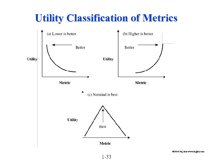 Utility Classification of Metrics © 2006 Raj Jain www. rajjain. com 1 -33
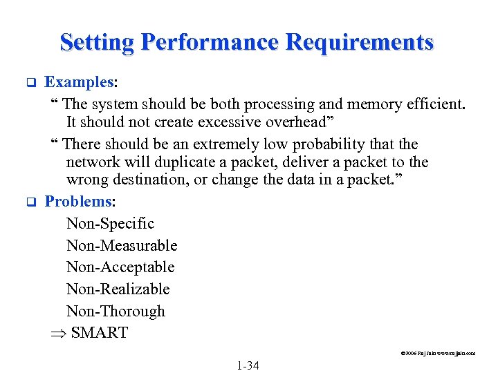 Setting Performance Requirements q q Examples: “ The system should be both processing and memory efficient. It should not create excessive overhead” “ There should be an extremely low probability that the network will duplicate a packet, deliver a packet to the wrong destination, or change the data in a packet. ” Problems: Non-Specific Non-Measurable Non-Acceptable Non-Realizable Non-Thorough SMART © 2006 Raj Jain www. rajjain. com 1 -34
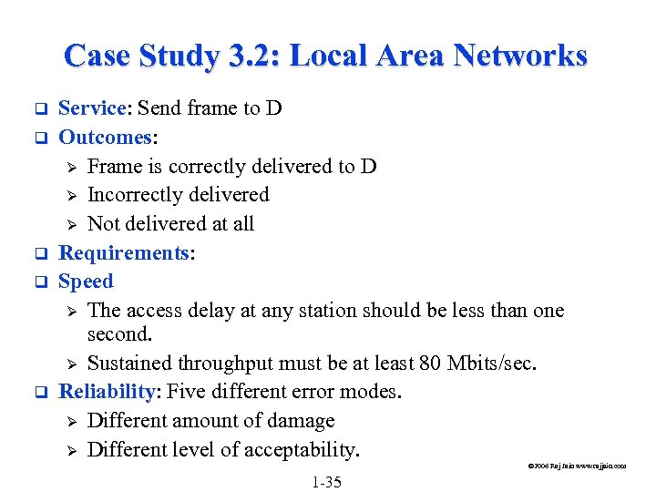 Case Study 3. 2: Local Area Networks q q q Service: Send frame to D Outcomes: Ø Frame is correctly delivered to D Ø Incorrectly delivered Ø Not delivered at all Requirements: Speed Ø The access delay at any station should be less than one second. Ø Sustained throughput must be at least 80 Mbits/sec. Reliability: Five different error modes. Ø Different amount of damage Ø Different level of acceptability. © 2006 Raj Jain www. rajjain. com 1 -35
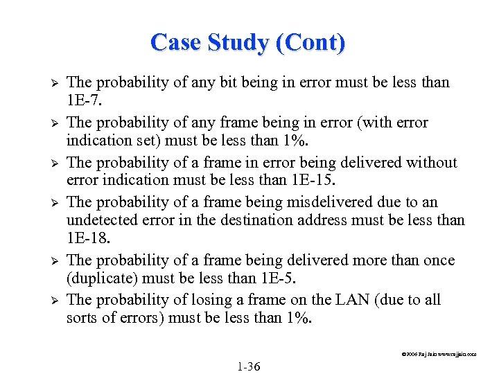 Case Study (Cont) Ø Ø Ø The probability of any bit being in error must be less than 1 E-7. The probability of any frame being in error (with error indication set) must be less than 1%. The probability of a frame in error being delivered without error indication must be less than 1 E-15. The probability of a frame being misdelivered due to an undetected error in the destination address must be less than 1 E-18. The probability of a frame being delivered more than once (duplicate) must be less than 1 E-5. The probability of losing a frame on the LAN (due to all sorts of errors) must be less than 1%. © 2006 Raj Jain www. rajjain. com 1 -36
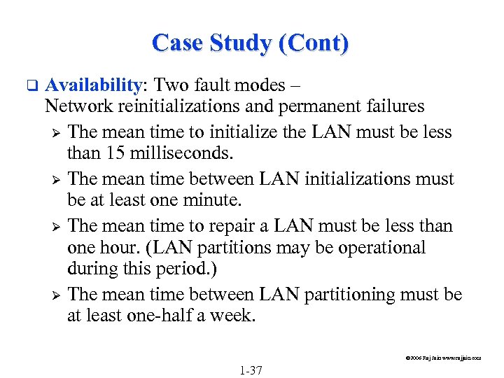 Case Study (Cont) q Availability: Two fault modes – Network reinitializations and permanent failures Ø The mean time to initialize the LAN must be less than 15 milliseconds. Ø The mean time between LAN initializations must be at least one minute. Ø The mean time to repair a LAN must be less than one hour. (LAN partitions may be operational during this period. ) Ø The mean time between LAN partitioning must be at least one-half a week. © 2006 Raj Jain www. rajjain. com 1 -37
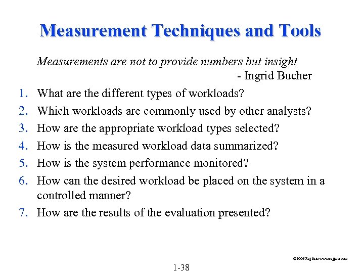 Measurement Techniques and Tools 1. 2. 3. 4. 5. 6. 7. Measurements are not to provide numbers but insight - Ingrid Bucher What are the different types of workloads? Which workloads are commonly used by other analysts? How are the appropriate workload types selected? How is the measured workload data summarized? How is the system performance monitored? How can the desired workload be placed on the system in a controlled manner? How are the results of the evaluation presented? © 2006 Raj Jain www. rajjain. com 1 -38
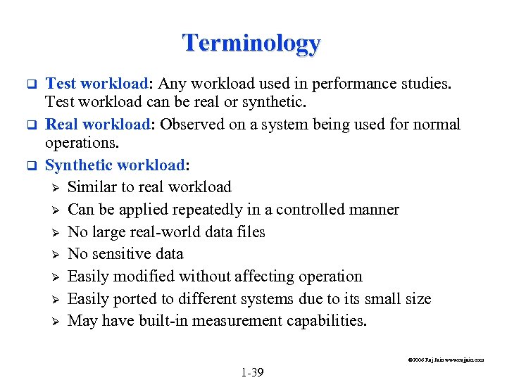 Terminology q q q Test workload: Any workload used in performance studies. Test workload can be real or synthetic. Real workload: Observed on a system being used for normal operations. Synthetic workload: Ø Similar to real workload Ø Can be applied repeatedly in a controlled manner Ø No large real-world data files Ø No sensitive data Ø Easily modified without affecting operation Ø Easily ported to different systems due to its small size Ø May have built-in measurement capabilities. © 2006 Raj Jain www. rajjain. com 1 -39
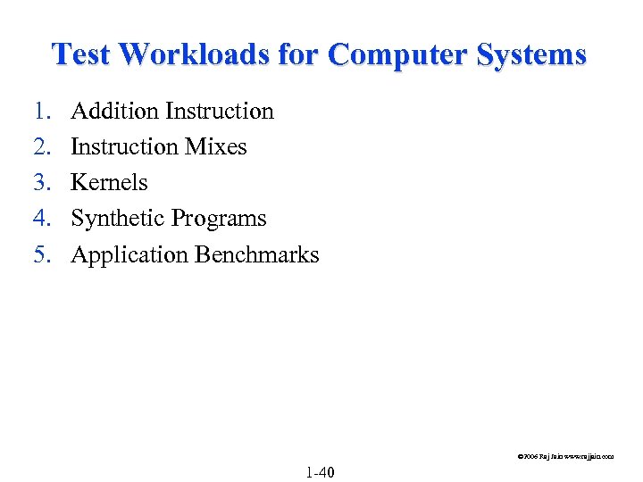 Test Workloads for Computer Systems 1. 2. 3. 4. 5. Addition Instruction Mixes Kernels Synthetic Programs Application Benchmarks © 2006 Raj Jain www. rajjain. com 1 -40
 Addition Instruction Processors were the most expensive and most used components of the system q Addition was the most frequent instruction q © 2006 Raj Jain www. rajjain. com 1 -41
 Instruction Mixes q q Instruction mix = instructions + usage frequency Gibson mix: Developed by Jack C. Gibson in 1959 for IBM 704 systems. © 2006 Raj Jain www. rajjain. com 1 -42
 Instruction Mixes (Cont) q q Disadvantages: Ø Complex classes of instructions not reflected in the mixes. Ø Instruction time varies with: q Addressing modes q Cache hit rates q Pipeline efficiency q Interference from other devices during processormemory access cycles q Parameter values q Frequency of zeros as a parameter q The distribution of zero digits in a multiplier q The average number of positions of preshift in floatingpoint add q Number of times a conditional branch is taken © 2006 Raj Jain www. rajjain. com 1 -43
 Instruction Mixes (Cont) q Performance Metrics: Ø MIPS = Millions of Instructions Per Second Ø MFLOPS = Millions of Floating Point Operations Per Second © 2006 Raj Jain www. rajjain. com 1 -44
 Kernels Kernel = nucleus q Kernel= the most frequent function q Commonly used kernels: Sieve, Puzzle, Tree Searching, Ackerman's Function, Matrix Inversion, and Sorting. q Disadvantages: Do not make use of I/O devices q © 2006 Raj Jain www. rajjain. com 1 -45
 Synthetic Programs To measure I/O performance lead analysts ) Exerciser loops q The first exerciser loop was by Buchholz (1969) who called it a synthetic program. q A Sample Exerciser: See program listing Figure 4. 1 in the book q © 2006 Raj Jain www. rajjain. com 1 -46
 Synthetic Programs q q Advantage: Ø Quickly developed and given to different vendors. Ø No real data files Ø Easily modified and ported to different systems. Ø Have built-in measurement capabilities Ø Measurement process is automated Ø Repeated easily on successive versions of the operating systems Disadvantages: Ø Too small Ø Do not make representative memory or disk references Ø Mechanisms for page faults and disk cache may not be adequately exercised. Ø CPU-I/O overlap may not be representative. Ø Loops may create synchronizations ) better or worse performance. © 2006 Raj Jain www. rajjain. com 1 -47
 Application Benchmarks For a particular industry: Debit-Credit for Banks q Benchmark = workload (Except instruction mixes) q Some Authors: Benchmark = set of programs taken from real workloads q Popular Benchmarks q © 2006 Raj Jain www. rajjain. com 1 -48
 Sieve Based on Eratosthenes' sieve algorithm: find all prime numbers below a given number n. q Algorithm: Ø Write down all integers from 1 to n Ø Strike out all multiples of k, for k=2, 3, …, n. q Example: Ø Write down all numbers from 1 to 20. Mark all as prime: 1, 2, 3, 4, 5, 6, 7, 8, 9, 10, 11, 12, 13, 14, 15, 16, 17, 18, 19, 20 q Remove all multiples of 2 from the list of primes: 1, 2, 3, 4, 5, 6, 7, 8, 9, 10, 11, 12, 13, 14, 15, 16, 17, 18, 19, 20 q © 2006 Raj Jain www. rajjain. com 1 -49
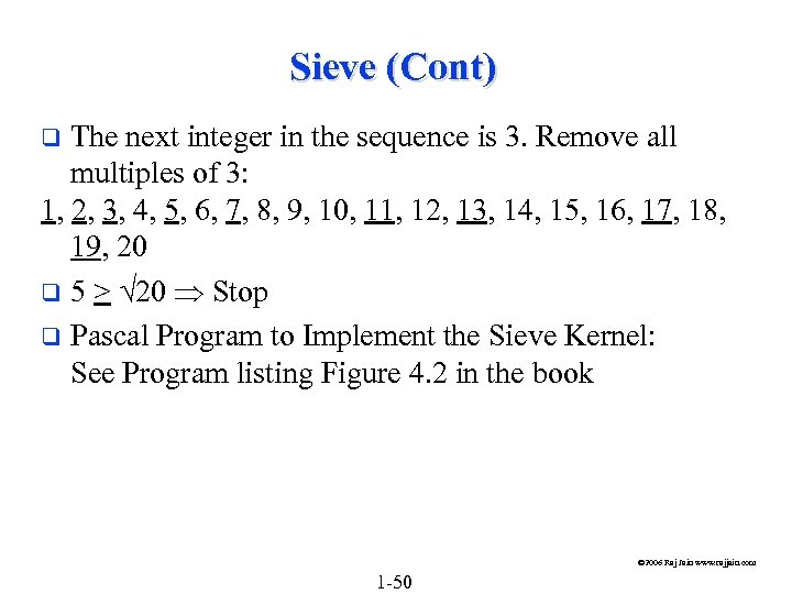 Sieve (Cont) The next integer in the sequence is 3. Remove all multiples of 3: 1, 2, 3, 4, 5, 6, 7, 8, 9, 10, 11, 12, 13, 14, 15, 16, 17, 18, 19, 20 q 5 > 20 Stop q Pascal Program to Implement the Sieve Kernel: See Program listing Figure 4. 2 in the book q © 2006 Raj Jain www. rajjain. com 1 -50
 Other Benchmarks Whetstone q U. S. Steel q LINPACK q Dhrystone q Doduc q TOP q Lawrence Livermore Loops q Digital Review Labs q Abingdon Cross Image-Processing Benchmark q © 2006 Raj Jain www. rajjain. com 1 -51
 SPEC Benchmark Suite q q Systems Performance Evaluation Cooperative (SPEC): Nonprofit corporation formed by leading computer vendors to develop a standardized set of benchmarks. Release 1. 0 consists of the following 10 benchmarks: GCC, Espresso, Spice 2 g 6, Doduc, LI, Eqntott, Matrix 300, Fpppp, Tomcatv Primarily stress the CPU, Floating Point Unit (FPU), and to some extent the memory subsystem To compare CPU speeds. Benchmarks to compare I/O and other subsystems may be included in future releases. © 2006 Raj Jain www. rajjain. com 1 -52
 SPEC (Cont) q q q The elapsed time to run two copies of a benchmark on each of the N processors of a system (a total of 2 N copies) is measured and compared with the time to run two copies of the benchmark on a reference system (which is VAX-11/780 for Release 1. 0). For each benchmark, the ratio of the time on the system under test and the reference system is reported as SPECthruput using a notation of #CPU@Ratio. For example, a system with three CPUs taking 1/15 times as long as the reference system on GCC benchmark has a SPECthruput of 3@15. Measure of the per processor throughput relative to the reference system © 2006 Raj Jain www. rajjain. com 1 -53
 SPEC (Cont) q q The aggregate throughput for all processors of a multiprocessor system can be obtained by multiplying the ratio by the number of processors. For example, the aggregate throughput for the above system is 45. The geometric mean of the SPECthruputs for the 10 benchmarks is used to indicate the overall performance for the suite and is called SPECmark. © 2006 Raj Jain www. rajjain. com 1 -54
 The Art of Workload Selection q q q Services Exercised Ø Example: Timesharing Systems Ø Example: Networks Ø Example: Magnetic Tape Backup System Level of Detail Representativeness Timeliness Other Considerations in Workload Selection © 2006 Raj Jain www. rajjain. com 1 -55
 The Art of Workload Selection Considerations: q Services exercised q Level of detail q Loading level q Impact of other components q Timeliness © 2006 Raj Jain www. rajjain. com 1 -56
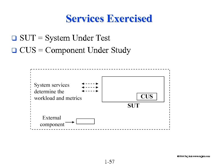 Services Exercised SUT = System Under Test q CUS = Component Under Study q © 2006 Raj Jain www. rajjain. com 1 -57
 Services Exercised (Cont) q q Do not confuse SUT w CUS Metrics depend upon SUT: MIPS is ok for two CPUs but not for two timesharing systems. Workload: depends upon the system. Examples: Ø CPU: instructions Ø System: Transactions Ø Transactions not good for CPU and vice versa Ø Two systems identical except for CPU q Comparing Systems: Use transactions q Comparing CPUs: Use instructions Ø Multiple services: Exercise as complete a set of services as possible. © 2006 Raj Jain www. rajjain. com 1 -58
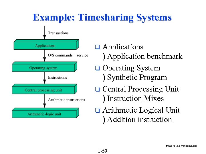 Example: Timesharing Systems Applications ) Application benchmark q Operating System ) Synthetic Program q Central Processing Unit ) Instruction Mixes q Arithmetic Logical Unit ) Addition instruction q © 2006 Raj Jain www. rajjain. com 1 -59
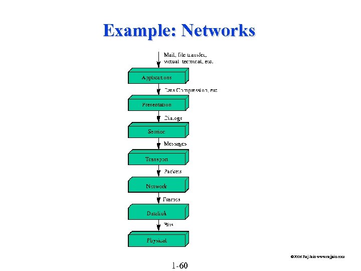 Example: Networks © 2006 Raj Jain www. rajjain. com 1 -60
 Level of Detail (Cont) q q q Average resource demand Ø Used for analytical modeling Ø Grouped similar services in classes Distribution of resource demands Ø Used if variance is large Ø Used if the distribution impacts the performance Workload used in simulation and analytical modeling: Ø Non executable: Used in analytical/simulation modeling Ø Executable workload: can be executed directly on a system © 2006 Raj Jain www. rajjain. com 1 -61
 Representativeness The test workload and real workload should have the same: q Elapsed Time q Resource Demands q Resource Usage Profile: Sequence and the amounts in which different resources are used. © 2006 Raj Jain www. rajjain. com 1 -62
 Timeliness Users are a moving target. q New systems new workloads q Users tend to optimize the demand. q Fast multiplication Higher frequency of multiplication instructions. q Important to monitor user behavior on an ongoing basis. q © 2006 Raj Jain www. rajjain. com 1 -63
 Other Considerations in Workload Selection q q q Loading Level: A workload may exercise a system to its: Ø Full capacity (best case) Ø Beyond its capacity (worst case) Ø At the load level observed in real workload (typical case). Ø For procurement purposes Typical Ø For design best to worst, all cases Impact of External Components: Ø Do not use a workload that makes external component a bottleneck All alternatives in the system give equally good performance. Repeatability © 2006 Raj Jain www. rajjain. com 1 -64
 Workload Characterization Techniques q q q Terminology Components and Parameter Selection Workload Characterization Techniques: Averaging, Single Parameter Histograms, Multi-parameter Histograms, Principal Component Analysis, Markov Models, Clustering Method: Minimum Spanning Tree, Nearest Centroid Problems with Clustering © 2006 Raj Jain www. rajjain. com 1 -65
 Terminology q User = Entity that makes the service request Workload components: Ø Applications Ø Sites Ø User Sessions q Workload parameters or Workload features: Measured quantities, service requests, or resource demands. For example: transaction types, instructions, packet sizes, source-destinations of a packet, and page reference pattern. q © 2006 Raj Jain www. rajjain. com 1 -66
 Components and Parameter Selection The workload component should be at the SUT interface. q Each component should represent as homogeneous a group as possible. Combining very different users into a site workload may not be meaningful. q Domain of the control affects the component: Example: mail system designer are more interested in determining a typical mail session than a typical user session. q Do not use parameters that depend upon the system, e. g. , the elapsed time, CPU time. q © 2006 Raj Jain www. rajjain. com 1 -67
 Components (Cont) Characteristics of service requests: Ø Arrival Time Ø Type of request or the resource demanded Ø Duration of the request Ø Quantity of the resource demanded, for example, pages of memory q Exclude those parameters that have little impact. q © 2006 Raj Jain www. rajjain. com 1 -68
 Workload Characterization Techniques 1. 2. 3. 4. 5. 6. Averaging Single-Parameter Histograms Multi-parameter Histograms Principal Component Analysis Markov Models Clustering © 2006 Raj Jain www. rajjain. com 1 -69
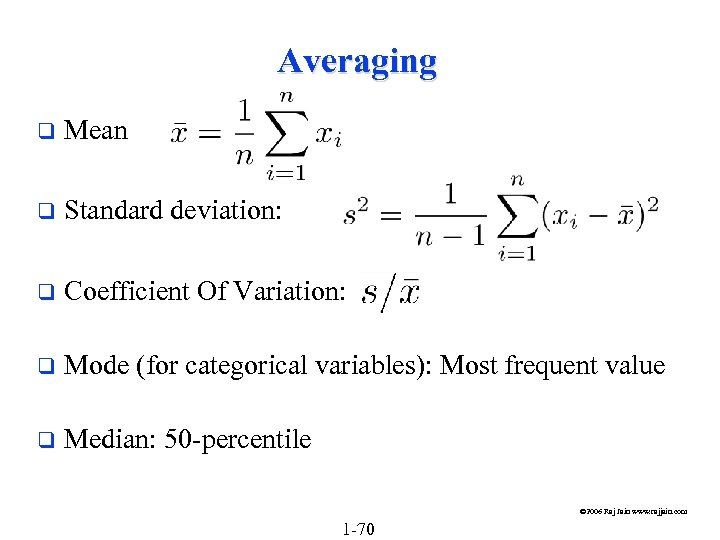 Averaging q Mean q Standard deviation: q Coefficient Of Variation: q Mode (for categorical variables): Most frequent value q Median: 50 -percentile © 2006 Raj Jain www. rajjain. com 1 -70
 Case Study: Program Usage in Educational Environments q High Coefficient of Variation © 2006 Raj Jain www. rajjain. com 1 -71
 Characteristics of an Average Editing Session q Reasonable variation © 2006 Raj Jain www. rajjain. com 1 -72
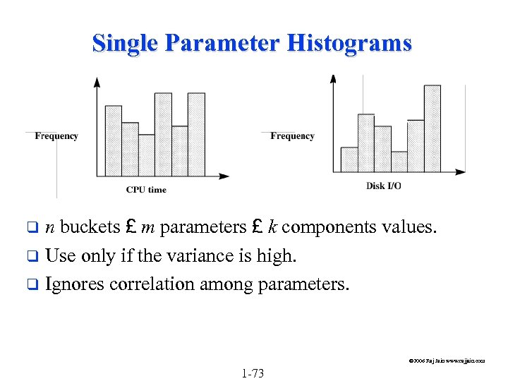 Single Parameter Histograms n buckets £ m parameters £ k components values. q Use only if the variance is high. q Ignores correlation among parameters. q © 2006 Raj Jain www. rajjain. com 1 -73
 Multi-parameter Histograms q Difficult to plot joint histograms for more than two parameters. © 2006 Raj Jain www. rajjain. com 1 -74
 Principal Component Analysis Key Idea: Use a weighted sum of parameters to classify the components. q Let xij denote the ith parameter for jth component. q yj = åi=1 n wi xij Principal component analysis assigns weights wi's such that yj's provide the maximum discrimination among the components. q The quantity yj is called the principal factor. q The factors are ordered. First factor explains the highest percentage of the variance. q © 2006 Raj Jain www. rajjain. com 1 -75
 Principal Component Analysis (Cont) q Statistically: Ø The y's are linear combinations of x's: yi = åj=1 n aij xj Here, aij is called the loading of variable xj on factor yi. The y's form an orthogonal set, that is, their inner product is zero:
 Finding Principal Factors Find the correlation matrix. q Find the eigen values of the matrix and sort them in the order of decreasing magnitude. q Find corresponding eigen vectors. These give the required loadings. q © 2006 Raj Jain www. rajjain. com 1 -77
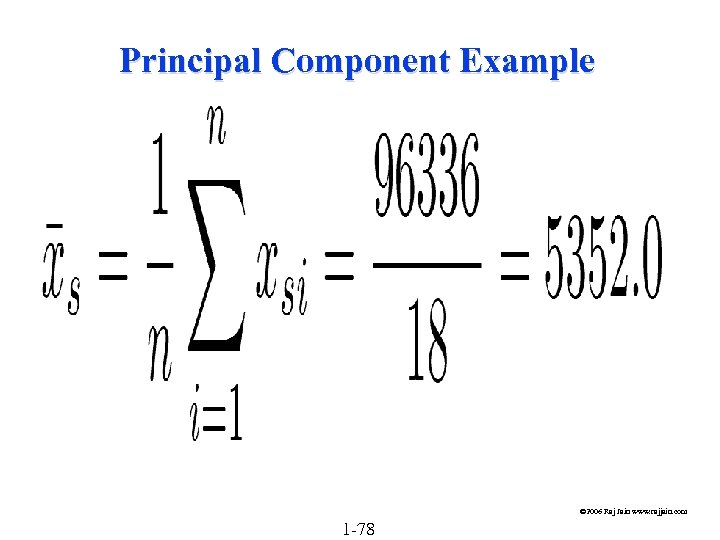 Principal Component Example © 2006 Raj Jain www. rajjain. com 1 -78
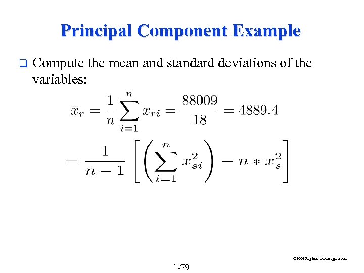 Principal Component Example q Compute the mean and standard deviations of the variables: © 2006 Raj Jain www. rajjain. com 1 -79
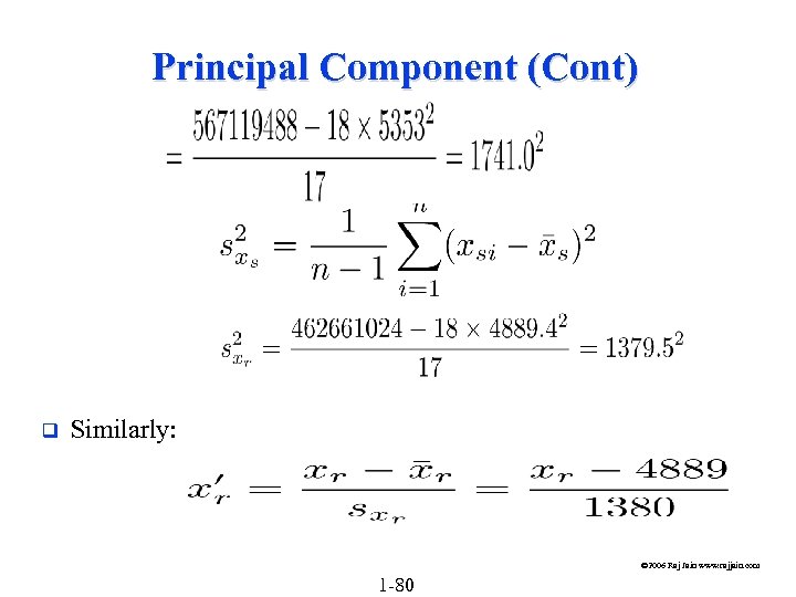 Principal Component (Cont) q Similarly: © 2006 Raj Jain www. rajjain. com 1 -80
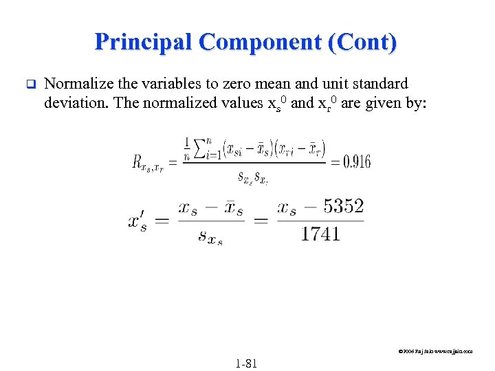 Principal Component (Cont) q Normalize the variables to zero mean and unit standard deviation. The normalized values xs 0 and xr 0 are given by: © 2006 Raj Jain www. rajjain. com 1 -81
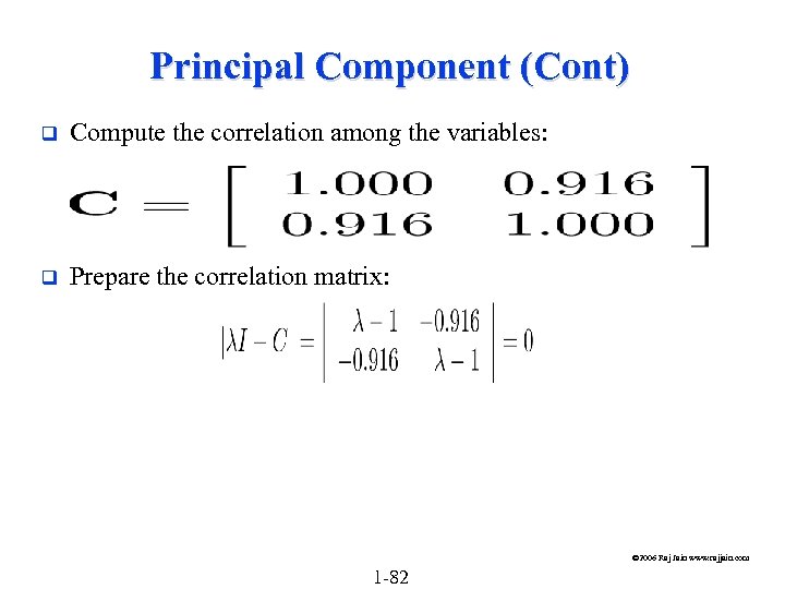 Principal Component (Cont) q Compute the correlation among the variables: q Prepare the correlation matrix: © 2006 Raj Jain www. rajjain. com 1 -82
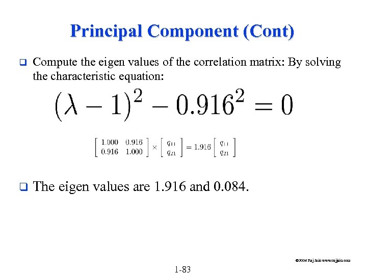 Principal Component (Cont) q Compute the eigen values of the correlation matrix: By solving the characteristic equation: q The eigen values are 1. 916 and 0. 084. © 2006 Raj Jain www. rajjain. com 1 -83
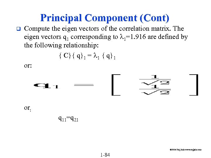 Principal Component (Cont) q Compute the eigen vectors of the correlation matrix. The eigen vectors q 1 corresponding to l 1=1. 916 are defined by the following relationship: { C}{ q}1 = l 1 { q}1 or: q 11=q 21 © 2006 Raj Jain www. rajjain. com 1 -84
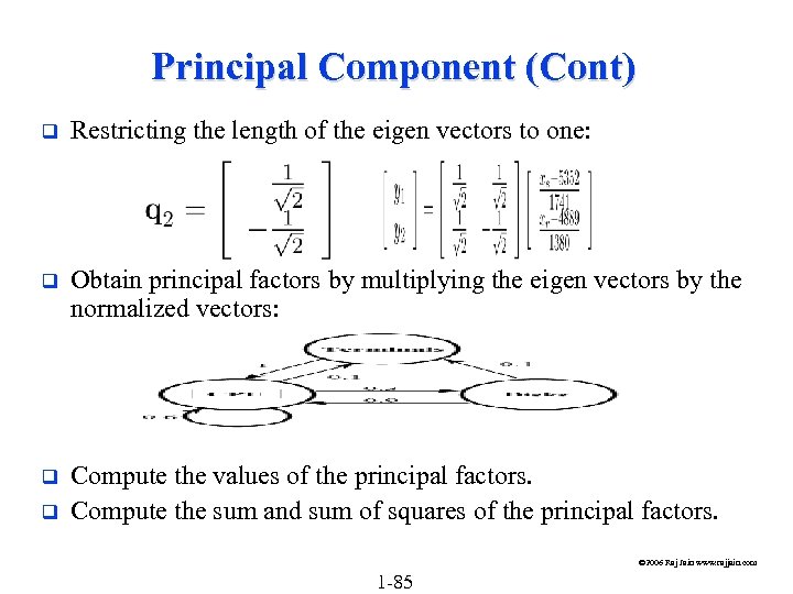 Principal Component (Cont) q Restricting the length of the eigen vectors to one: q Obtain principal factors by multiplying the eigen vectors by the normalized vectors: q Compute the values of the principal factors. Compute the sum and sum of squares of the principal factors. q © 2006 Raj Jain www. rajjain. com 1 -85
 Principal Component (Cont) The sum must be zero. q The sum of squares give the percentage of variation explained. q © 2006 Raj Jain www. rajjain. com 1 -86
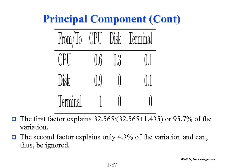 Principal Component (Cont) q q The first factor explains 32. 565/(32. 565+1. 435) or 95. 7% of the variation. The second factor explains only 4. 3% of the variation and can, thus, be ignored. © 2006 Raj Jain www. rajjain. com 1 -87
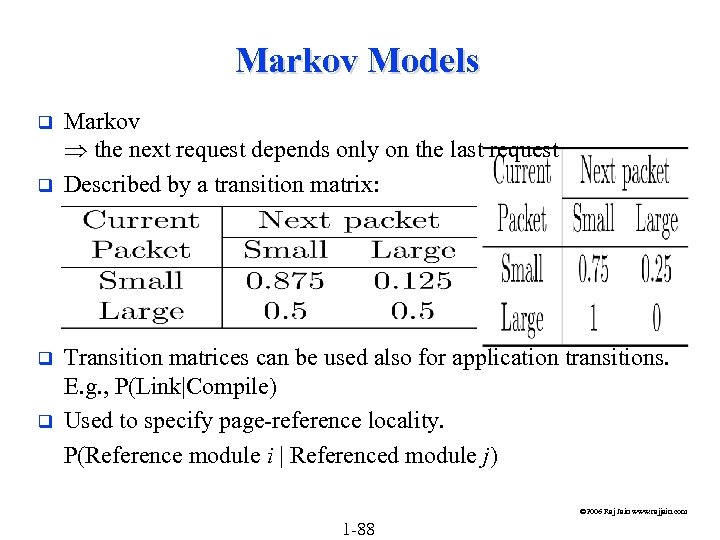 Markov Models q q Markov the next request depends only on the last request Described by a transition matrix: Transition matrices can be used also for application transitions. E. g. , P(Link|Compile) Used to specify page-reference locality. P(Reference module i | Referenced module j) © 2006 Raj Jain www. rajjain. com 1 -88
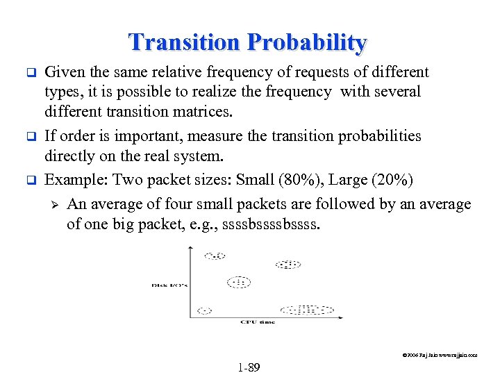 Transition Probability q q q Given the same relative frequency of requests of different types, it is possible to realize the frequency with several different transition matrices. If order is important, measure the transition probabilities directly on the real system. Example: Two packet sizes: Small (80%), Large (20%) Ø An average of four small packets are followed by an average of one big packet, e. g. , ssssbssss. © 2006 Raj Jain www. rajjain. com 1 -89
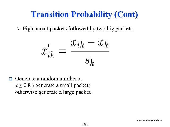 Transition Probability (Cont) Ø q Eight small packets followed by two big packets. Generate a random number x. x < 0. 8 ) generate a small packet; otherwise generate a large packet. © 2006 Raj Jain www. rajjain. com 1 -90
 Clustering © 2006 Raj Jain www. rajjain. com 1 -91
 Clustering Steps 1. 2. 3. 4. 5. 6. 7. 8. Take a sample, that is, a subset of workload components. Select workload parameters. Select a distance measure. Remove outliers. Scale all observations. Perform clustering. Interpret results. Change parameters, or number of clusters, and repeat steps 3 -7. 9. Select representative components from each cluster. © 2006 Raj Jain www. rajjain. com 1 -92
 1. Sampling In one study, 2% of the population was chosen for analysis; later 99% of the population could be assigned to the clusters obtained. q Random selection q Select top consumers of a resource. q © 2006 Raj Jain www. rajjain. com 1 -93
 2. Parameter Selection Criteria: Ø Impact on performance Ø Variance q Method: Redo clustering with one less parameter q Principal component analysis: Identify parameters with the highest variance. q © 2006 Raj Jain www. rajjain. com 1 -94
 3. Transformation q If the distribution is highly skewed, consider a function of the parameter, e. g. , log of CPU time © 2006 Raj Jain www. rajjain. com 1 -95
 4. Outliers = data points with extreme parameter values q Affect normalization q Can exclude only if that do not consume a significant portion of the system resources. Example, backup. q © 2006 Raj Jain www. rajjain. com 1 -96
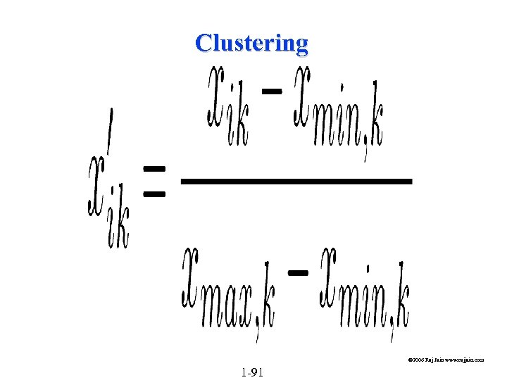
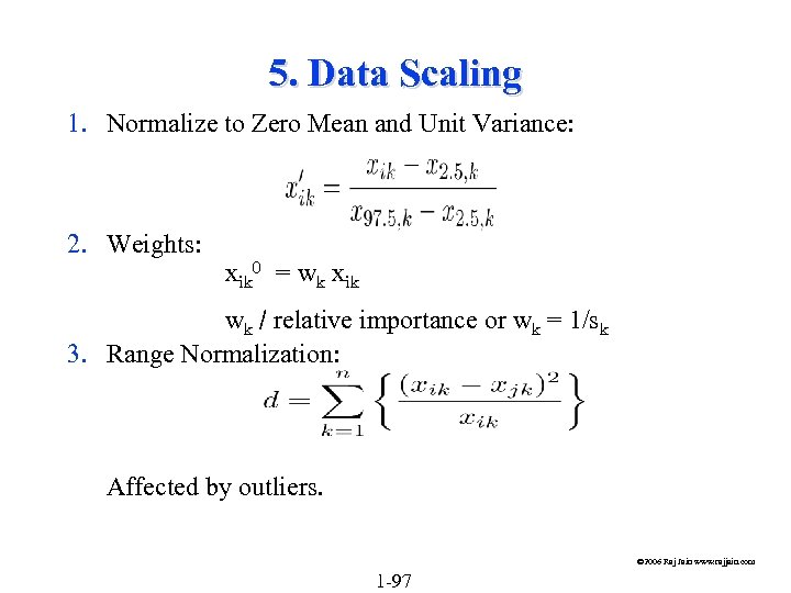 5. Data Scaling 1. Normalize to Zero Mean and Unit Variance: 2. Weights: xik 0 = wk xik wk / relative importance or wk = 1/sk 3. Range Normalization: Affected by outliers. © 2006 Raj Jain www. rajjain. com 1 -97
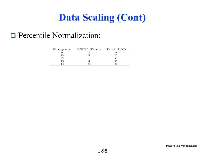 Data Scaling (Cont) q Percentile Normalization: © 2006 Raj Jain www. rajjain. com 1 -98
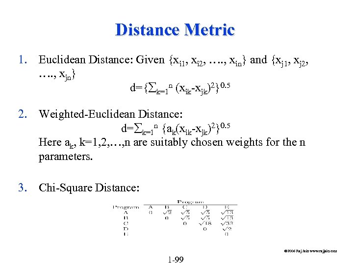 Distance Metric 1. Euclidean Distance: Given {xi 1, xi 2, …. , xin} and {xj 1, xj 2, …. , xjn} d={åk=1 n (xik-xjk)2}0. 5 2. Weighted-Euclidean Distance: d=åk=1 n {ak(xik-xjk)2}0. 5 Here ak, k=1, 2, …, n are suitably chosen weights for the n parameters. 3. Chi-Square Distance: © 2006 Raj Jain www. rajjain. com 1 -99
 Distance Metric (Cont) q The Euclidean distance is the most commonly used distance metric. q The weighted Euclidean is used if the parameters have not been scaled or if the parameters have significantly different levels of importance. q Use Chi-Square distance only if x. k's are close to each other. Parameters with low values of x. k get higher weights. © 2006 Raj Jain www. rajjain. com 1 -100
 Clustering Techniques Goal: Partition into groups so the members of a group are as similar as possible and different groups are as dissimilar as possible. q Statistically, the intragroup variance should be as small as possible, and inter-group variance should be as large as possible. Total Variance = Intra-group Variance + Inter-group Variance q © 2006 Raj Jain www. rajjain. com 1 -101
 Clustering Techniques (Cont) Nonhierarchical techniques: Start with an arbitrary set of k clusters, Move members until the intra-group variance is minimum. q Hierarchical Techniques: Ø Agglomerative: Start with n clusters and merge Ø Divisive: Start with one cluster and divide. q Two popular techniques: Ø Minimum spanning tree method (agglomerative) Ø Centroid method (Divisive) q © 2006 Raj Jain www. rajjain. com 1 -102
 Minimum Spanning Tree-Clustering Method 1. 2. 3. 4. 5. Start with k = n clusters. Find the centroid of the ith cluster, i=1, 2, …, k. Compute the inter-cluster distance matrix. Merge the nearest clusters. Repeat steps 2 through 4 until all components are part of one cluster. © 2006 Raj Jain www. rajjain. com 1 -103
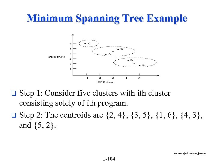 Minimum Spanning Tree Example Step 1: Consider five clusters with cluster consisting solely of ith program. q Step 2: The centroids are {2, 4}, {3, 5}, {1, 6}, {4, 3}, and {5, 2}. q © 2006 Raj Jain www. rajjain. com 1 -104
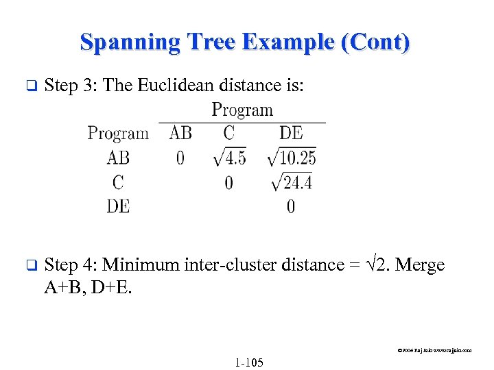 Spanning Tree Example (Cont) q Step 3: The Euclidean distance is: q Step 4: Minimum inter-cluster distance = 2. Merge A+B, D+E. © 2006 Raj Jain www. rajjain. com 1 -105
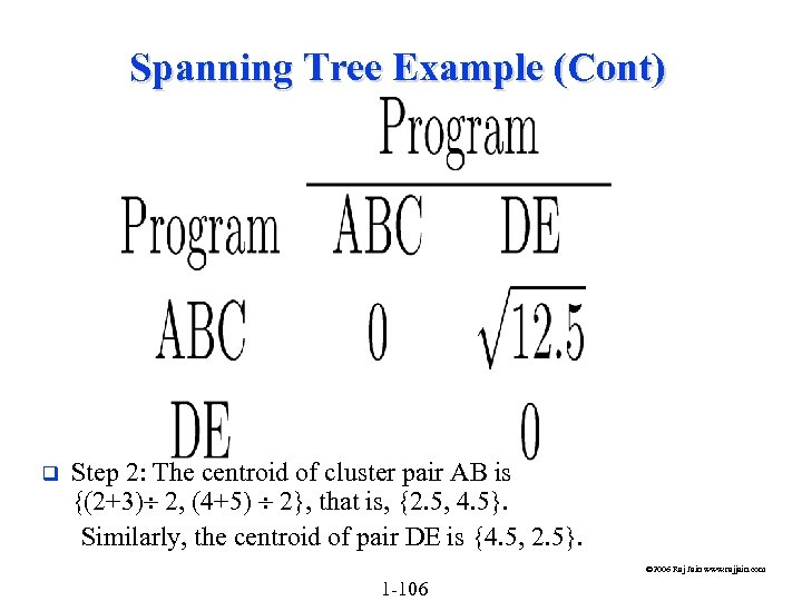 Spanning Tree Example (Cont) q Step 2: The centroid of cluster pair AB is {(2+3) 2, (4+5) 2}, that is, {2. 5, 4. 5}. Similarly, the centroid of pair DE is {4. 5, 2. 5}. © 2006 Raj Jain www. rajjain. com 1 -106
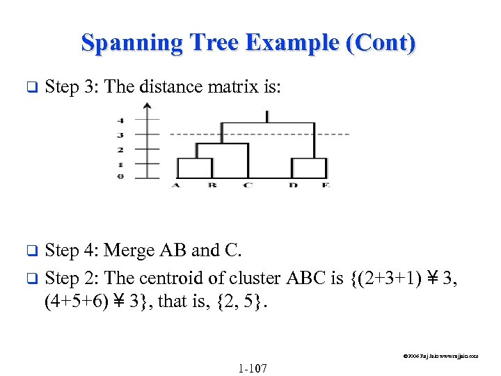 Spanning Tree Example (Cont) q Step 3: The distance matrix is: Step 4: Merge AB and C. q Step 2: The centroid of cluster ABC is {(2+3+1) ¥ 3, (4+5+6) ¥ 3}, that is, {2, 5}. q © 2006 Raj Jain www. rajjain. com 1 -107
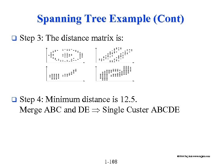 Spanning Tree Example (Cont) q Step 3: The distance matrix is: q Step 4: Minimum distance is 12. 5. Merge ABC and DE Single Custer ABCDE © 2006 Raj Jain www. rajjain. com 1 -108
 Dendogram q q Dendogram = Spanning Tree Purpose: Obtain clusters for any given maximum allowable intra-cluster distance. © 2006 Raj Jain www. rajjain. com 1 -109
 Nearest Centroid Method q q q Start with k = 1. Find the centroid and intra-cluster variance for ith cluster, i= 1, 2, …, k. Find the cluster with the highest variance and arbitrarily divide it into two clusters. Ø Find the two components that are farthest apart, assign other components according to their distance from these points. Ø Place all components below the centroid in one cluster and all components above this hyper plane in the other. Adjust the points in the two new clusters until the inter-cluster distance between the two clusters is maximum. Set k = k+1. Repeat steps 2 through 4 until k = n. © 2006 Raj Jain www. rajjain. com 1 -110
 Cluster Interpretation Assign all measured components to the clusters. q Clusters with very small populations and small total resource demands can be discarded. (Don't just discard a small cluster) q Interpret clusters in functional terms, e. g. , a business application, Or label clusters by their resource demands, for example, CPU-bound, I/O-bound, and so forth. q Select one or more representative components from each cluster for use as test workload. q © 2006 Raj Jain www. rajjain. com 1 -111
 Problems with Clustering © 2006 Raj Jain www. rajjain. com 1 -112
 Problems with Clustering (Cont) Goal: Minimize variance. q The results of clustering are highly variable. No rules for: Ø Selection of parameters Ø Distance measure Ø Scaling q Labeling each cluster by functionality is difficult. Ø In one study, editing programs appeared in 23 different clusters. q Requires many repetitions of the analysis. q © 2006 Raj Jain www. rajjain. com 1 -113


