CSCE 932 Spring 2007 Test Generation for Combinational

CSCE 932, Spring 2007 Test Generation for Combinational Logic 1

Outline Fundamental Concepts Structure vs. Function Boolean Difference Test Generation Algorithms Multi-valued Algebras Complexity of test generation PODEM Boolean-Satisfiability Based Summary 2

Origins of Stuck-Faults Eldred (1959) – First use of structural testing for the Honeywell Datamatic 1000 computer Galey, Norby, Roth (1961) – First publication of stuck-at-0 and stuck-at-1 faults Seshu & Freeman (1962) – Use of stuck-faults for parallel fault simulation Poage (1963) – Theoretical analysis of stuck-at faults 3

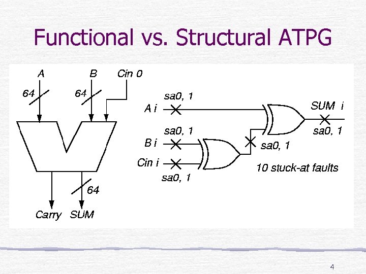
Functional vs. Structural ATPG 4

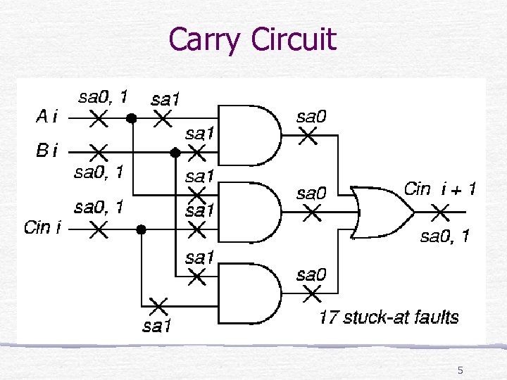
Carry Circuit 5

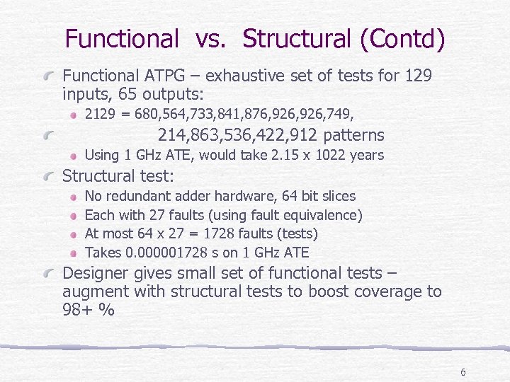
Functional vs. Structural (Contd) Functional ATPG – exhaustive set of tests for 129 inputs, 65 outputs: 2129 = 680, 564, 733, 841, 876, 926, 749, 214, 863, 536, 422, 912 patterns Using 1 GHz ATE, would take 2. 15 x 1022 years Structural test: No redundant adder hardware, 64 bit slices Each with 27 faults (using fault equivalence) At most 64 x 27 = 1728 faults (tests) Takes 0. 000001728 s on 1 GHz ATE Designer gives small set of functional tests – augment with structural tests to boost coverage to 98+ % 6

Boolean Difference I will illustrate the concepts in class, along with illustrative examples. 7

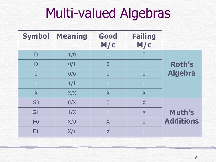
Multi-valued Algebras Symbol Meaning Good M/c Failing M/c D 1/0 1 0 D 0/1 0 0/0 0 0 1 1/1 1 1 X X/X X X G 0 0/X 0 X G 1 1/X 1 X F 0 X/0 X 0 F 1 X/1 X 1 Roth’s Algebra Muth’s Additions 8

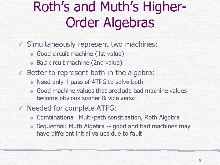
Roth’s and Muth’s Higher. Order Algebras Simultaneously represent two machines: Good circuit machine (1 st value) Bad circuit machine (2 nd value) Better to represent both in the algebra: Need only 1 pass of ATPG to solve both Good machine values that preclude bad machine values become obvious sooner & vice versa Needed for complete ATPG: Combinational: Multi-path sensitization, Roth Algebra Sequential: Muth Algebra -- good and bad machines may have different initial values due to fault 9

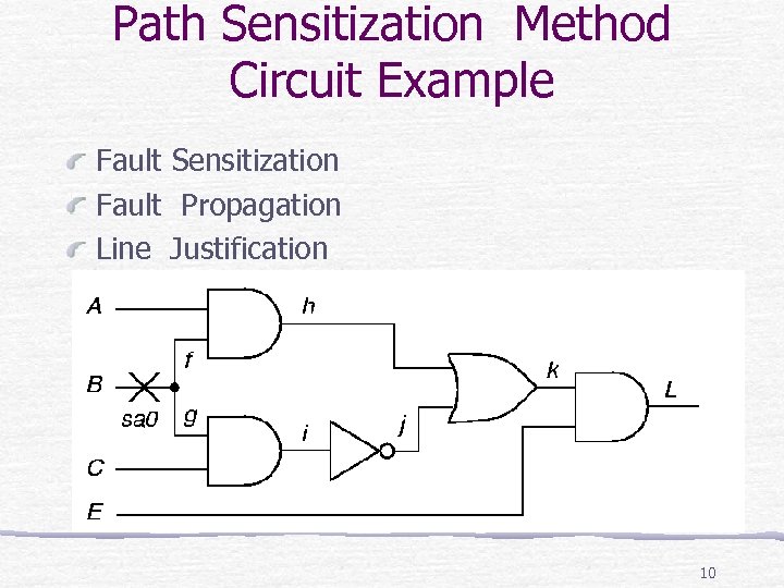
Path Sensitization Method Circuit Example Fault Sensitization Fault Propagation Line Justification 10

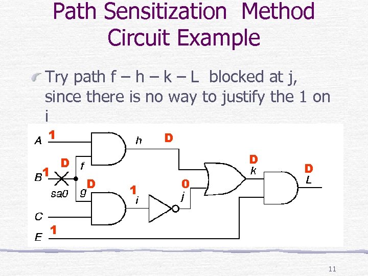
Path Sensitization Method Circuit Example Try path f – h – k – L blocked at j, since there is no way to justify the 1 on i 1 1 D D 1 0 D 1 11

Path Sensitization Method Circuit Example Try simultaneous paths f – h – k – L and g – i – j – k – L blocked at k because D-frontier (chain of D or D) disappears 1 1 D D D 1 12

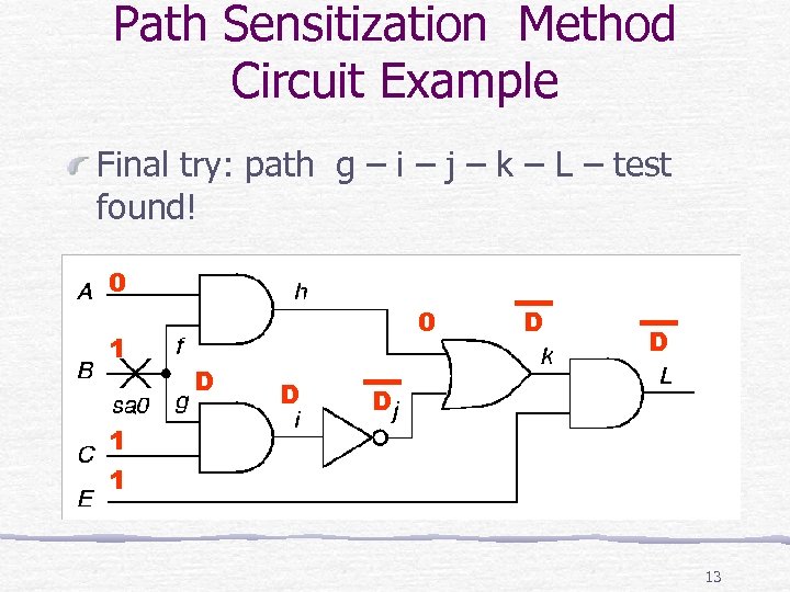
Path Sensitization Method Circuit Example Final try: path g – i – j – k – L – test found! 0 1 0 D D D 1 1 13

Complexity of Test Generation The primary source of complexity is that the number of sensitizable paths grow exponentially with the circuit size and in the worst case the algorithm may have to search all of them for a solution. 14

Algorithmic Complexity of Test Generation Algorithmic complexity refers to the worstcase-time behavior in terms of problem parameter(s) For combinational test generation, circuit size (in number of lines) is used as the parameter. Sahni and Ibarra* showed NP-completeness of test generation by reducing a well NPcomplete problem (3 -SAT) to the combinational test-generation problem. O. H. Ibarra and S. K. Sahni, “Polynomially Complete Fault Detection Problems, ” IEEE Trans. Computers, March 1975, pp. 242 -249/ 15

PODEM Test Generation Algorithm Structure-based and fault oriented Signal values are explicitly assigned at the PIs only; other values are computed by implication Eliminates D-algorithm’s need to justify internal signals Backtracks at PIs only when a contradiction occurs Many extensions exist with more complex heuristics, e. g. the FAN algorithm 16

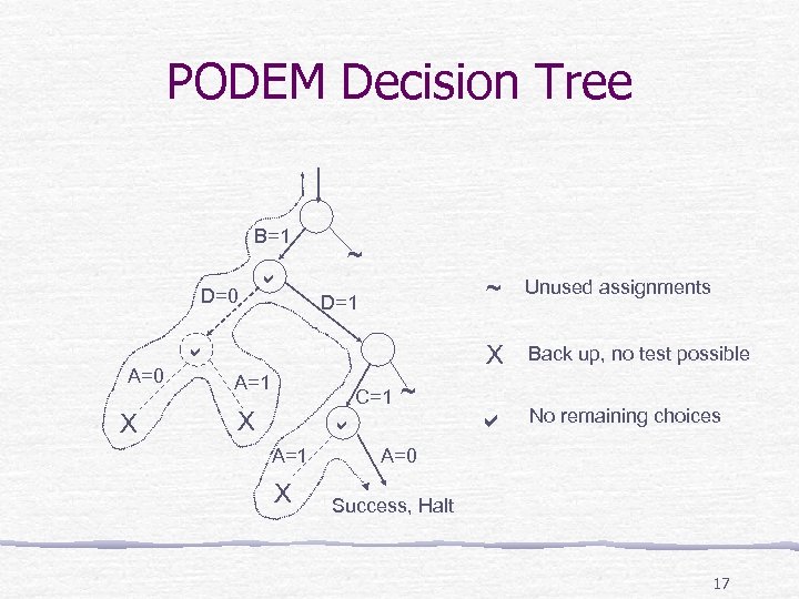
PODEM Decision Tree B=1 X ~ D=1 a A=1 C=1 X X Back up, no test possible ~ a A=1 Unused assignments X D=0 A=0 a ~ a No remaining choices A=0 Success, Halt 17

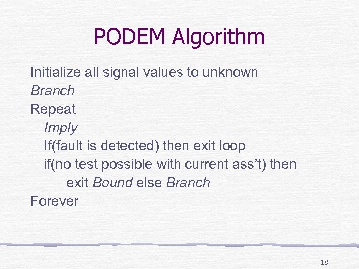
PODEM Algorithm Initialize all signal values to unknown Branch Repeat Imply If(fault is detected) then exit loop if(no test possible with current ass’t) then exit Bound else Branch Forever 18

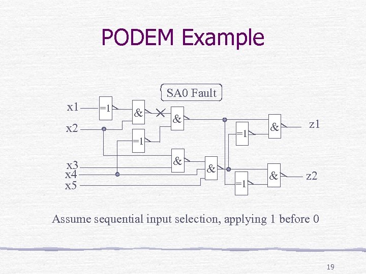
PODEM Example SA 0 Fault x 1 =1 & x 2 & =1 =1 x 3 x 4 x 5 & & =1 & z 2 Assume sequential input selection, applying 1 before 0 19

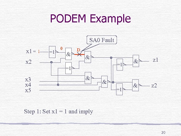
PODEM Example SA 0 Fault x 1 =1 0 & x 2 D & =1 =1 x 3 x 4 x 5 & & =1 & z 2 Step 1: Set x 1 = 1 and imply 20

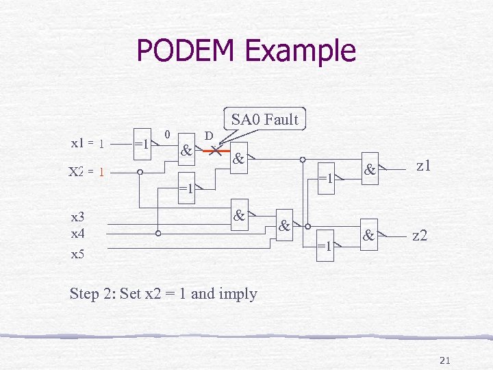
PODEM Example x 1 =1 0 SA 0 Fault & X 2 = 1 D & =1 =1 x 3 x 4 x 5 & & =1 & z 2 Step 2: Set x 2 = 1 and imply 21

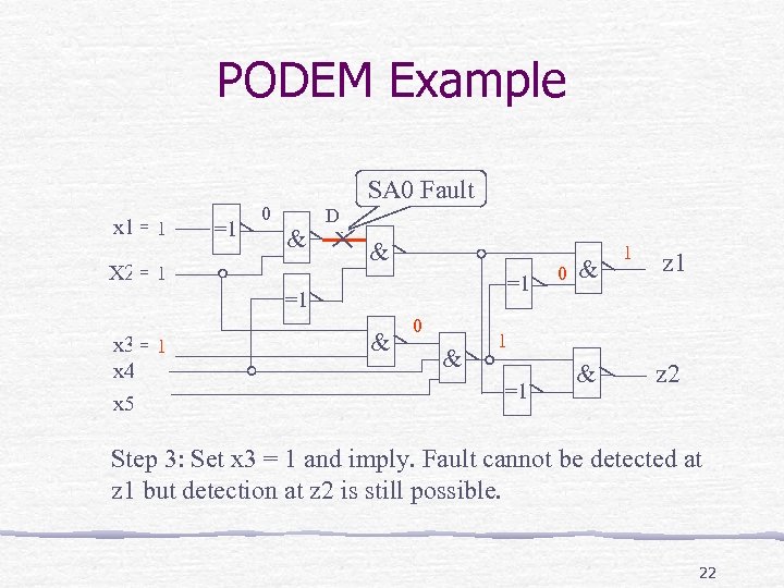
PODEM Example x 1 =1 0 SA 0 Fault & X 2 = 1 D & =1 =1 x 3 = 1 x 4 x 5 & 0 & 1 z 1 1 =1 & z 2 Step 3: Set x 3 = 1 and imply. Fault cannot be detected at z 1 but detection at z 2 is still possible. 22

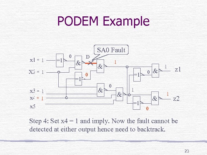
PODEM Example x 1 =1 0 SA 0 Fault & X 2 = 1 =1 x 3 = 1 x 4 = 1 x 5 D 1 & =1 0 & 0 & 1 =1 & 1 1 z 2 0 Step 4: Set x 4 = 1 and imply. Now the fault cannot be detected at either output hence need to backtrack. 23

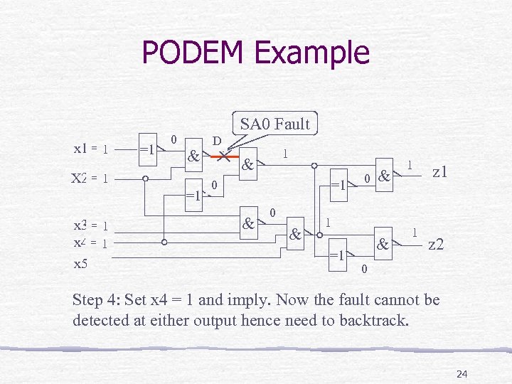
PODEM Example x 1 =1 0 SA 0 Fault & X 2 = 1 =1 x 3 = 1 x 4 = 1 x 5 D 1 & =1 0 & 0 & 1 =1 & 1 1 z 2 0 Step 4: Set x 4 = 1 and imply. Now the fault cannot be detected at either output hence need to backtrack. 24

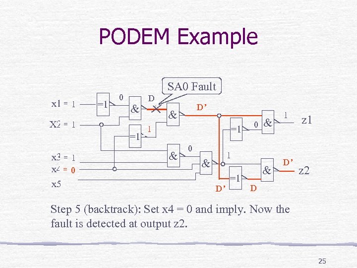
PODEM Example x 1 =1 0 SA 0 Fault & X 2 = 1 =1 x 3 = 1 x 4 = 0 x 5 D D’ & =1 1 & 0 0 & 1 & D’ =1 & 1 D’ z 1 z 2 D Step 5 (backtrack): Set x 4 = 0 and imply. Now the fault is detected at output z 2. 25

Podem Heuristics Several heuristics are used for speedup Line objectives Selecting alternatives in back-tracing Selecting alternatives for extending D-path to an observable output Many heuristics are based on the controllability and absorbability estimates for lines in the circuit 26

Boolean Satisfiability Given a Boolean formula in CNF (productof-sums), determine if there is an assignment of variable values that satisfies the formula. Special Cases: 2 -SAT: CNF clauses have at most 2 literals 3 -SAT: CNF clauses have at most 3 literals 27

Test Generation as a Boolean Satisfiability Problem 1. Gate Representation (AND Gate Example): Express C = AB in conjunctive normal form (CNF). The formula is true iff the values of A, B, and C are consistent with the AND function. 2. Circuit Representation: Logically AND the CNF for each gate. The resulting formula, in CNF, is true all the signal values are consistent. 3. Construct the Boolean difference circuit for the target fault (next slide). 4. Represent the Boolean difference circuit by its CNF formula and set the signal at its output to 1. An input assignment is a test iff it satisfies the CNF. 28

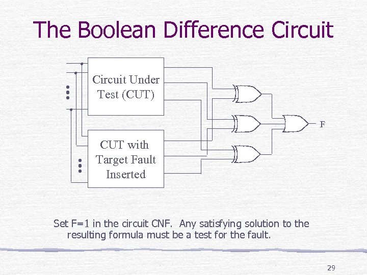
The Boolean Difference Circuit Under Test (CUT) F CUT with Target Fault Inserted Set F=1 in the circuit CNF. Any satisfying solution to the resulting formula must be a test for the fault. 29

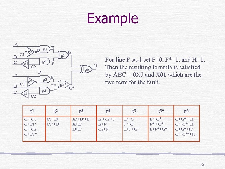
Example A g 2 B C 1 C g 1 E D g 3 g 4 C 2 G F g 6 D A B C g 5 C 1 g 2 g 1 g 3 E F* g 5* G* g 4 F H For line F sa-1 set F=0, F*=1, and H=1. Then the resulting formula is satisfied by ABC = 0 X 0 and X 01 which are the two tests for the fault. C 2 g 1 C’+C 1 C+C 1’ C’+C 2 C+C 2” g 2 C 1+D C 1’+D’ g 3 g 4 A’+D’+E A+E’ D+E’ B’+c 2’+F B+F’ C 2+F’ g 5 E’+G F’+G E+F+G’ g 5* E’+G* F*’+G* E+F*+G*’ g 6 G+G*’+H G’+G*+H G+G*+H’ G’+G*’+H’ 30

SAT Solvers The DPLL Algorithm: Davis-Putnam [JACM 7(1) 1960], and Davis-Putnam-Longemann-Loveland [CACM May 1962] The line justification step in PODEM [Goel, IEEE TC, March 1981] can also be used as a SAT solver The DPLL algorithm has been enhanced in chaff [Moskewicz et al. DAC 2001] and implemented in mchaff and zchaff, the latter being the most widely known and used. Other SAT solvers to note: GRASP [Marques-Silva and Sakalla, IEEE TC, May 1999], SATO [Zhang, Int. Conf. Automated Deduction, 1997] Generally, the DPLL enhancements try to improve on the original backtrack algorithm through careful engineering of all aspects of the search 31

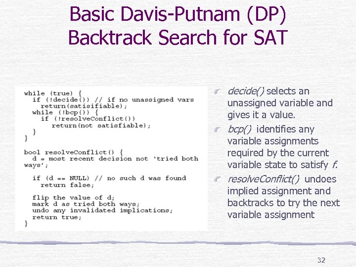
Basic Davis-Putnam (DP) Backtrack Search for SAT decide() selects an unassigned variable and gives it a value. bcp() identifies any variable assignments required by the current variable state to satisfy f. resolve. Conflict() undoes implied assignment and backtracks to try the next variable assignment 32

2 -SAT Based SAT Solving The boolean satisfiability problem for binary clauses (2 -SAT) is polynomially solvable while 3 -SAT and the general satisfiability problem is NP-complete. This suggests another heuristic of solving the satisfiability problem: generate and test solutions for the binary clauses against the whole CNF until success. 33

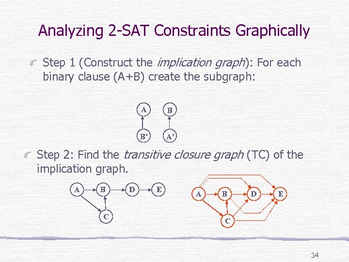
Analyzing 2 -SAT Constraints Graphically Step 1 (Construct the implication graph): For each binary clause (A+B) create the subgraph: A B B’ A’ Step 2: Find the transitive closure graph (TC) of the implication graph. A B C D E A B D E C 34

Analyzing 2 -SAT Constraints Graphically Step 3 (Analyze the transitive-closure graph): (Contradiction): Both (C’, C) and (C, C’) are in the TC. This implies C must be true and false at the same time. This would occur if the fault was redundant (untestable). (Fixed Signal Values): Only one of (C’, C) and (C, C’) is in the TC this implies C has a fixed binary value. (Identical Signal Values): If both (A’, B) and (A, B’) are in the TC then literals A and B must assume identical signal values. (Excluded Signal Value): If (A’, B) is in the TC and no other edges occur between these four literals, then the combination AB=10 is excluded from the solution. 35

Transitive Closure Test Generation Algorithm (TRAN)* In TRAN test generation is carried out entirely by dynamically updating the TC after each variable assignment and analyzing it. * See, Chakradhar et al. IEEE TCAD, June 1993 and Larrabee, TCAD, January 1992. 36

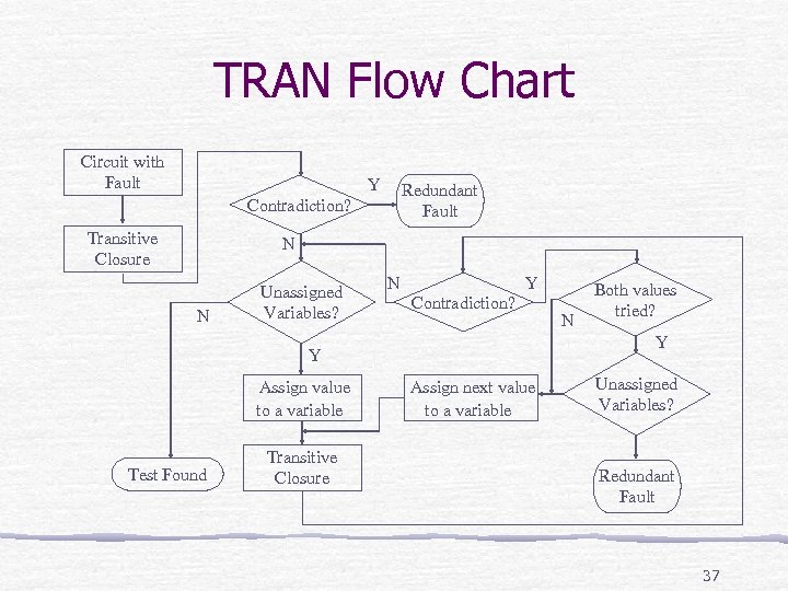
TRAN Flow Chart Circuit with Fault Y Redundant Fault Contradiction? Transitive Closure N N Unassigned Variables? N Y Contradiction? Y Y Assign value to a variable Test Found Transitive Closure N Both values tried? Assign next value to a variable Unassigned Variables? Redundant Fault 37

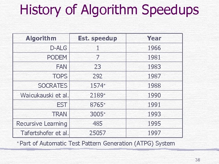
History of Algorithm Speedups Algorithm Est. speedup Year D-ALG 1 1966 PODEM 7 1981 FAN 23 1983 TOPS 292 1987 SOCRATES 1574* 1988 Waicukauski et al. 2189* 1990 EST 8765* 1991 TRAN 3005* 1993 485 1995 25057 1997 Recursive Learning Tafertshofer et al. * Part of Automatic Test Pattern Generation (ATPG) System 38

Test Generation for Sequential -Circuits 40

Time-Frame Expansion COMB LOGIC C M Iterative Logic Array (ILA) Representation Initial State COMB LOGIC C Clock Cycle 0 M COMB LOGIC C Clock Cycle 1 M COMB LOGIC C M Final State Clock Cycle 2 41

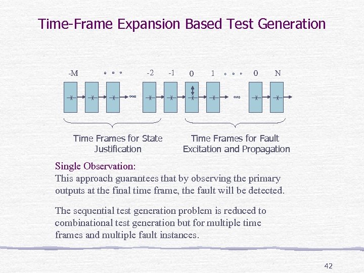
Time-Frame Expansion Based Test Generation -M -2 Time Frames for State Justification -1 0 N Time Frames for Fault Excitation and Propagation Single Observation: This approach guarantees that by observing the primary outputs at the final time frame, the fault will be detected. The sequential test generation problem is reduced to combinational test generation but for multiple time frames and multiple fault instances. 42

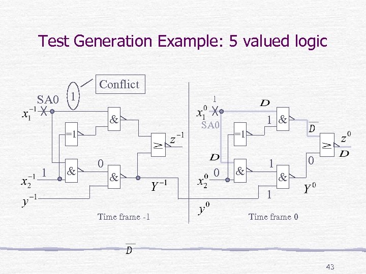
Test Generation Example: 5 valued logic SA 0 1 Conflict 1 & =1 1 & 0 & SA 0 0 1 & =1 & 0 1 & 1 Time frame -1 Time frame 0 43

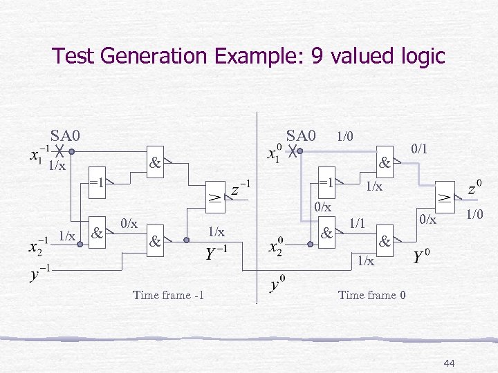
Test Generation Example: 9 valued logic SA 0 1/0 & 1/x & =1 =1 1/x 0/x 1/x & 0/x & 1/x & 0/1 1/0 0/x 1/1 & 1/x Time frame -1 Time frame 0 44

The “Reset Problem” Synchronizing sequence is a generalized reset for FSMs. It reduces the total uncertainty of the initial state to a known fixed state. However, the reduction in ambiguity for some FSMs may not be fast enough to find the synchronizing sequence by algorithmic means using 3 -valued logic. Consider the example machine (from Miczo’s text, p. 273) on the next page 45

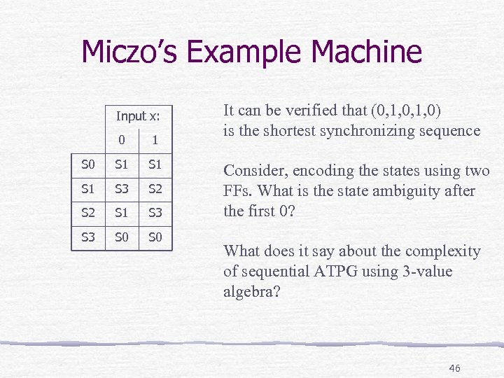
Miczo’s Example Machine Input x: 0 1 S 0 S 1 S 1 S 3 S 2 S 1 S 3 S 0 It can be verified that (0, 1, 0) is the shortest synchronizing sequence Consider, encoding the states using two FFs. What is the state ambiguity after the first 0? What does it say about the complexity of sequential ATPG using 3 -value algebra? 46

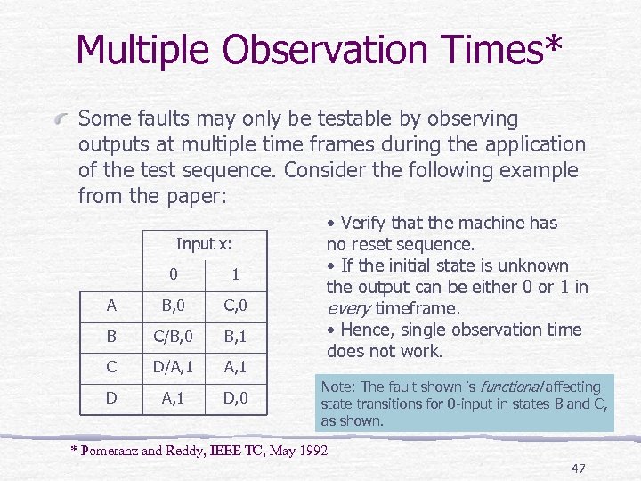
Multiple Observation Times* Some faults may only be testable by observing outputs at multiple time frames during the application of the test sequence. Consider the following example from the paper: Input x: 0 1 A B, 0 C, 0 B C/B, 0 B, 1 C D/A, 1 D, 0 • Verify that the machine has no reset sequence. • If the initial state is unknown the output can be either 0 or 1 in every timeframe. • Hence, single observation time does not work. Note: The fault shown is functional affecting state transitions for 0 -input in states B and C, as shown. * Pomeranz and Reddy, IEEE TC, May 1992 47

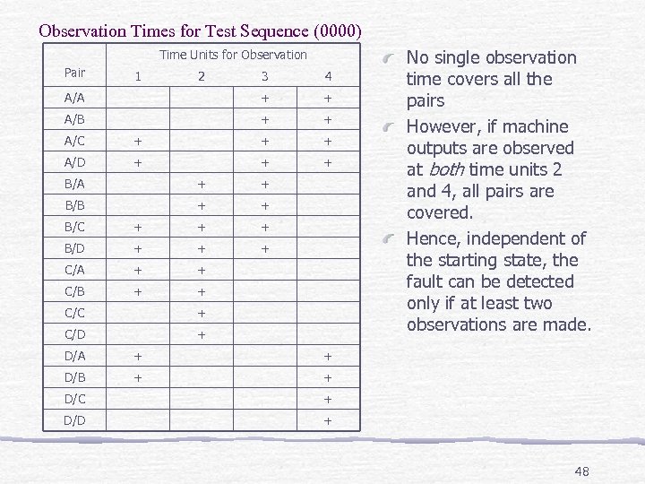
Observation Times for Test Sequence (0000) Time Units for Observation Pair 1 2 3 4 A/A + + A/B + + A/C + + + A/D + + + B/A + + B/B + + B/C + + + B/D + + + C/A + + C/B + + C/C + C/D + D/A + + D/B + No single observation time covers all the pairs However, if machine outputs are observed at both time units 2 and 4, all pairs are covered. Hence, independent of the starting state, the fault can be detected only if at least two observations are made. + D/C + D/D + 48

Distinguishing Sequence in Finite State Machine Assume two copies of the same FSM, one starts in state s and the other in state t. A distinguishing sequence for states s and t is any input sequence that produces a different output. 49

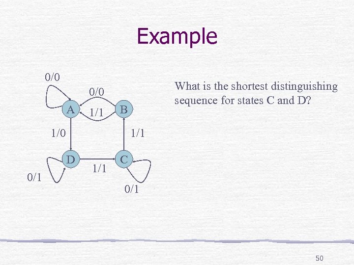
Example 0/0 What is the shortest distinguishing sequence for states C and D? 0/0 A 1/1 B 1/0 1/1 D 0/1 1/1 C 0/1 50

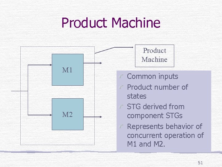
Product Machine M 1 M 2 Common inputs Product number of states STG derived from component STGs Represents behavior of concurrent operation of M 1 and M 2. 51

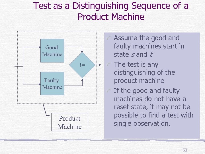
Test as a Distinguishing Sequence of a Product Machine Good Machine != Faulty Machine Product Machine Assume the good and faulty machines start in state s and t The test is any distinguishing of the product machine If the good and faulty machines do not have a reset state, it may not be possible to find a test with single observation. 52

Sequential Circuit ATPG Simulation-Based Methods Contrast with target-fault-based: Main loop starts with an initial sequence of test vectors (could be random or otherwise) The sequence is progressively modified and augmented based on simulation based evaluation of the testability of the current set, until the desired level of coverage is reached. IBM’s SOFTG* is an early example of this approach. * T. J. Snethen, “Simulator-Oriented Fault Test Generator, ” Proc. DAC, 1977, pp. 88 -93. 53

Other Simulation-Based Methods Contest Directed search Cost functions Genetic Algorithms Spectral Methods Summary 54

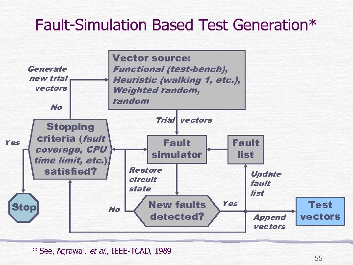
Fault-Simulation Based Test Generation* Generate new trial vectors No Yes Vector source: Functional (test-bench), Heuristic (walking 1, etc. ), Weighted random, random Trial vectors Stopping criteria (fault coverage, CPU time limit, etc. ) satisfied? Stop Fault simulator Fault list Restore circuit state No New faults detected? * See, Agrawal, et al. , IEEE-TCAD, 1989 Yes Update fault list Append vectors Test vectors 55

Sequential ATPG Summary Combinational ATPG algorithms are extended: Time-frame expansion unrolls time as combinational array Justification via backward time Nine-valued logic system Unlike combinational ATPG: Completeness not guaranteed using 3 -valued logic simulation Some circuits may require 9 -valued D-algebra 5 -valued is not enough Simulation-based ATPG may be a more attractive alternative Cycle-free circuits (where sequential elements don’t form a cycle through combinational logic) are much easier to test than cyclic circuits Require at most dseq time-frames Always initializable DFT a must for large circuits: Either full or partial scan. 60