f67f8f7ed2abb99390d8ed7d63210f22.ppt
- Количество слайдов: 134
 CS 490 D: Introduction to Data Mining Prof. Walid Aref January 30, 2004 Association Rules CS 490 D
 Mining Association Rules in Large Databases • Association rule mining • Algorithms for scalable mining of (singledimensional Boolean) association rules in transactional databases • Mining various kinds of association/correlation rules • Constraint-based association mining • Sequential pattern mining • Applications/extensions of frequent pattern mining • Summary CS 490 D 2
 What Is Association Mining? • Association rule mining: – Finding frequent patterns, associations, correlations, or causal structures among sets of items or objects in transaction databases, relational databases, and other information repositories. – Frequent pattern: pattern (set of items, sequence, etc. ) that occurs frequently in a database [AIS 93] • Motivation: finding regularities in data – What products were often purchased together? — Beer and diapers? ! – What are the subsequent purchases after buying a PC? – What kinds of DNA are sensitive to this new drug? – Can we automatically classify web documents? CS 490 D 3
 Why Is Association Mining Important? • Foundation for many essential data mining tasks – Association, correlation, causality – Sequential patterns, temporal or cyclic association, partial periodicity, spatial and multimedia association – Associative classification, cluster analysis, iceberg cube, fascicles (semantic data compression) • Broad applications – Basket data analysis, cross-marketing, catalog design, sale campaign analysis – Web log (click stream) analysis, DNA sequence analysis, etc. CS 490 D 4
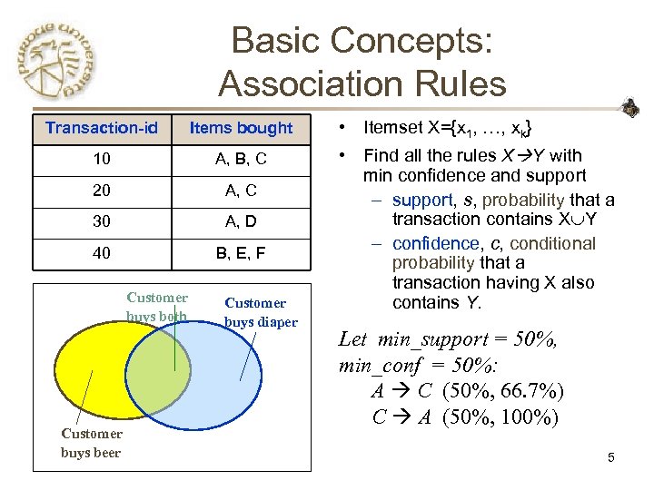 Basic Concepts: Association Rules Transaction-id Items bought 10 A, B, C 20 A, C 30 A, D 40 B, E, F Customer buys both Customer buys beer Customer buys diaper • Itemset X={x 1, …, xk} • Find all the rules X Y with min confidence and support – support, s, probability that a transaction contains X Y – confidence, c, conditional probability that a transaction having X also contains Y. Let min_support = 50%, min_conf = 50%: A C (50%, 66. 7%) C A (50%, 100%) 5
 Mining Association Rules: Example Min. support 50% Min. confidence 50% Transaction-id Items bought 10 A, B, C 20 A, C Frequent pattern Support 30 A, D {A} 75% 40 B, E, F {B} 50% {C} 50% {A, C} 50% For rule A C: support = support({A} {C}) = 50% confidence = support({A} {C})/support({A}) = 66. 6% CS 490 D 6
 Mining Association Rules: What We Need to Know • Goal: Rules with high support/confidence • How to compute? – Support: Find sets of items that occur frequently – Confidence: Find frequency of subsets of supported itemsets • If we have all frequently occurring sets of items (frequent itemsets), we can compute support and confidence! CS 490 D 7
 Mining Association Rules in Large Databases • Association rule mining • Algorithms for scalable mining of (singledimensional Boolean) association rules in transactional databases • Mining various kinds of association/correlation rules • Constraint-based association mining • Sequential pattern mining • Applications/extensions of frequent pattern mining • Summary CS 490 D 8
 Apriori: A Candidate Generationand-test Approach • Any subset of a frequent itemset must be frequent – if {beer, diaper, nuts} is frequent, so is {beer, diaper} – Every transaction having {beer, diaper, nuts} also contains {beer, diaper} • Apriori pruning principle: If there is any itemset which is infrequent, its superset should not be generated/tested! • Method: – generate length (k+1) candidate itemsets from length k frequent itemsets, and – test the candidates against DB • Performance studies show its efficiency and scalability • Agrawal & Srikant 1994, Mannila, et al. 1994 CS 490 D 9
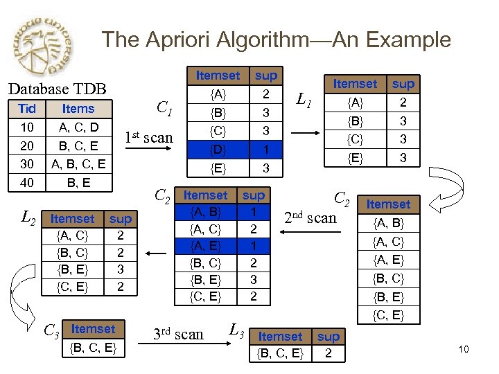 The Apriori Algorithm—An Example Database TDB Tid 10 20 30 40 L 2 C 1 Items A, C, D B, C, E A, B, C, E B, E Itemset {A, C} {B, E} {C, E} C 3 1 st scan sup 2 2 3 2 Itemset {B, C, E} Itemset {A} {B} {C} {D} {E} sup 2 3 3 1 3 L 1 Itemset {A} {B} {C} {E} sup 2 3 3 3 Frequency ≥ C 2 Itemset sup 50%, Confidence 100%: C 2 Itemset {A, B} 1 nd 2 A scan. C {A, B} {A, C} {A, E} {B, C} {B, E} {C, E} 3 rd scan 2 1 2 3 2 L 3 B E BC E CE B BE C Itemset {B, C, E} sup 2 {A, C} {A, E} {B, C} {B, E} {C, E} 10
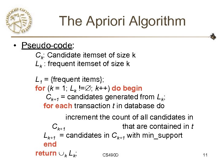 The Apriori Algorithm • Pseudo-code: Ck: Candidate itemset of size k Lk : frequent itemset of size k L 1 = {frequent items}; for (k = 1; Lk != ; k++) do begin Ck+1 = candidates generated from Lk; for each transaction t in database do increment the count of all candidates in Ck+1 that are contained in t Lk+1 = candidates in Ck+1 with min_support end return k Lk; CS 490 D 11
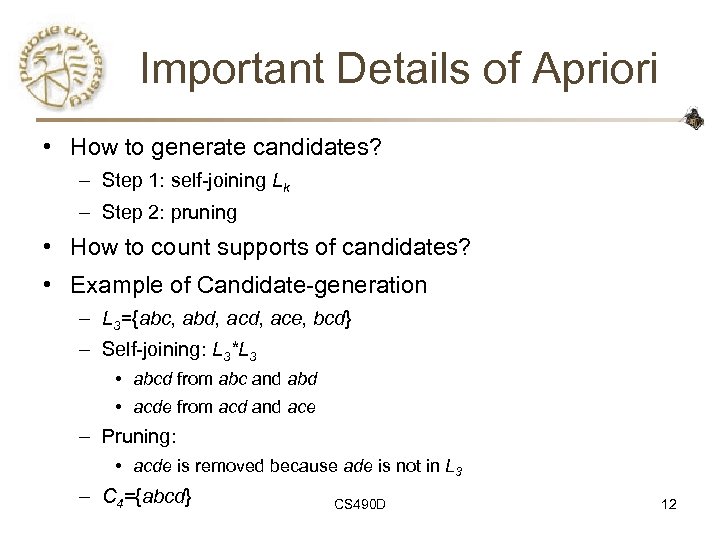 Important Details of Apriori • How to generate candidates? – Step 1: self-joining Lk – Step 2: pruning • How to count supports of candidates? • Example of Candidate-generation – L 3={abc, abd, ace, bcd} – Self-joining: L 3*L 3 • abcd from abc and abd • acde from acd and ace – Pruning: • acde is removed because ade is not in L 3 – C 4={abcd} CS 490 D 12
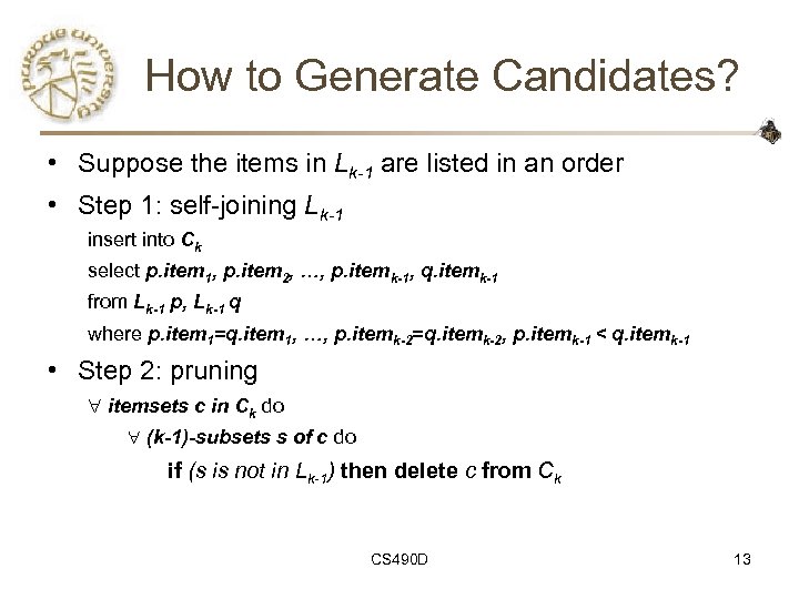 How to Generate Candidates? • Suppose the items in Lk-1 are listed in an order • Step 1: self-joining Lk-1 insert into Ck select p. item 1, p. item 2, …, p. itemk-1, q. itemk-1 from Lk-1 p, Lk-1 q where p. item 1=q. item 1, …, p. itemk-2=q. itemk-2, p. itemk-1 < q. itemk-1 • Step 2: pruning itemsets c in Ck do (k-1)-subsets s of c do if (s is not in Lk-1) then delete c from Ck CS 490 D 13
 How to Count Supports of Candidates? • Why counting supports of candidates a problem? – The total number of candidates can be very huge – One transaction may contain many candidates • Method: – Candidate itemsets are stored in a hash-tree – Leaf node of hash-tree contains a list of itemsets and counts – Interior node contains a hash table – Subset function: finds all the candidates contained in a transaction CS 490 D 14
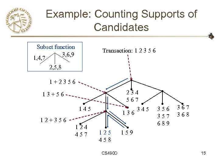 Example: Counting Supports of Candidates Subset function 3, 6, 9 1, 4, 7 Transaction: 1 2 3 5 6 2, 5, 8 1+2356 234 567 13+56 145 136 12+356 124 457 125 458 CS 490 D 345 356 357 689 367 368 159 15
 Efficient Implementation of Apriori in SQL • Hard to get good performance out of pure SQL (SQL-92) based approaches alone • Make use of object-relational extensions like UDFs, BLOBs, Table functions etc. – Get orders of magnitude improvement • S. Sarawagi, S. Thomas, and R. Agrawal. Integrating association rule mining with relational database systems: Alternatives and implications. In SIGMOD’ 98 CS 490 D 16
 Challenges of Frequent Pattern Mining • Challenges – Multiple scans of transaction database – Huge number of candidates – Tedious workload of support counting for candidates • Improving Apriori: general ideas – Reduce passes of transaction database scans – Shrink number of candidates – Facilitate support counting of candidates CS 490 D 17
 DIC: Reduce Number of Scans ABCD ABC ABD ACD BCD AB AC BC B A AD C BD D CD Apriori {} Itemset lattice S. Brin R. Motwani, J. Ullman, and S. Tsur. Dynamic itemset counting and implication rules for market basket data. In SIGMOD’ 97 • Once both A and D are determined frequent, the counting of AD begins • Once all length-2 subsets of BCD are determined frequent, the counting of BCD begins Transactions 1 -itemsets 2 -itemsets … 1 -itemsets 2 -items DIC 3 -items 18
 Partition: Scan Database Only Twice • Any itemset that is potentially frequent in DB must be frequent in at least one of the partitions of DB – Scan 1: partition database and find local frequent patterns – Scan 2: consolidate global frequent patterns • A. Savasere, E. Omiecinski, and S. Navathe. An efficient algorithm for mining association in large databases. In VLDB’ 95 CS 490 D 19
 CS 490 D: Introduction to Data Mining Prof. Chris Clifton February 2, 2004 Association Rules CS 490 D
 Sampling for Frequent Patterns • Select a sample of original database, mine frequent patterns within sample using Apriori • Scan database once to verify frequent itemsets found in sample, only borders of closure of frequent patterns are checked – Example: check abcd instead of ab, ac, …, etc. • Scan database again to find missed frequent patterns • H. Toivonen. Sampling large databases for association rules. In VLDB’ 96 CS 490 D 21
 DHP: Reduce the Number of Candidates • A k-itemset whose corresponding hashing bucket count is below the threshold cannot be frequent – – Candidates: a, b, c, d, e Hash entries: {ab, ad, ae} {bd, be, de} … Frequent 1 -itemset: a, b, d, e ab is not a candidate 2 -itemset if the sum of count of {ab, ad, ae} is below support threshold • J. Park, M. Chen, and P. Yu. An effective hashbased algorithm for mining association rules. In SIGMOD’ 95 CS 490 D 22
 Eclat/Max. Eclat and VIPER: Exploring Vertical Data Format • Use tid-list, the list of transaction-ids containing an itemset • Compression of tid-lists – Itemset A: t 1, t 2, t 3, sup(A)=3 – Itemset B: t 2, t 3, t 4, sup(B)=3 – Itemset AB: t 2, t 3, sup(AB)=2 • Major operation: intersection of tid-lists • M. Zaki et al. New algorithms for fast discovery of association rules. In KDD’ 97 • P. Shenoy et al. Turbo-charging vertical mining of large databases. In SIGMOD’ 00 CS 490 D 23
 Bottleneck of Frequent-pattern Mining • Multiple database scans are costly • Mining long patterns needs many passes of scanning and generates lots of candidates – To find frequent itemset i 1 i 2…i 100 • # of scans: 100 • # of Candidates: (1001) + (1002) + … + (110000) = 2100 -1 = 1. 27*1030 ! • Bottleneck: candidate-generation-and-test • Can we avoid candidate generation? CS 490 D 24
 Mining Frequent Patterns Without Candidate Generation • Grow long patterns from short ones using local frequent items – “abc” is a frequent pattern – Get all transactions having “abc”: DB|abc – “d” is a local frequent item in DB|abc abcd is a frequent pattern CS 490 D 25
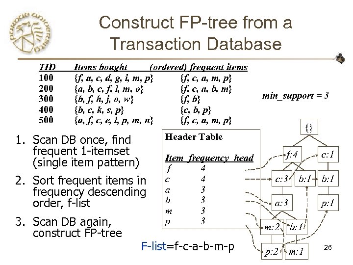 Construct FP-tree from a Transaction Database TID 100 200 300 400 500 Items bought (ordered) frequent items {f, a, c, d, g, i, m, p} {f, c, a, m, p} {a, b, c, f, l, m, o} {f, c, a, b, m} {b, f, h, j, o, w} {f, b} {b, c, k, s, p} {c, b, p} {a, f, c, e, l, p, m, n} {f, c, a, m, p} {} Header Table 1. Scan DB once, find frequent 1 -itemset (single item pattern) 2. Sort frequent items in frequency descending order, f-list 3. Scan DB again, construct FP-tree min_support = 3 Item frequency head f 4 c 4 a 3 b 3 m 3 p 3 F-list=f-c-a-b-m-p f: 4 c: 3 c: 1 b: 1 a: 3 b: 1 p: 1 m: 2 b: 1 p: 2 m: 1 26
 Benefits of the FP-tree Structure • Completeness – Preserve complete information for frequent pattern mining – Never break a long pattern of any transaction • Compactness – Reduce irrelevant info—infrequent items are gone – Items in frequency descending order: the more frequently occurring, the more likely to be shared – Never be larger than the original database (not count node-links and the count field) – For Connect-4 DB, compression ratio could be over 100 CS 490 D 27
 Partition Patterns and Databases • Frequent patterns can be partitioned into subsets according to f-list – F-list=f-c-a-b-m-p – Patterns containing p – Patterns having m but no p –… – Patterns having c but no a nor b, m, p – Pattern f • Completeness and non-redundency CS 490 D 28
 Find Patterns Having P From Pconditional Database • Starting at the frequent item header table in the FP-tree • Traverse the FP-tree by following the link of each frequent item p • Accumulate all of transformed prefix paths of item p to form p’s conditional pattern base {} Header Table Item frequency head f 4 c 4 a 3 b 3 m 3 p 3 f: 4 c: 1 Conditional pattern bases b: 1 a: 3 b: 1 p: 1 cond. pattern base c f: 3 a fc: 3 b c: 3 item fca: 1, f: 1, c: 1 m: 2 b: 1 m fca: 2, fcab: 1 p: 2 m: 1 p fcam: 2, cb: 1 CS 490 D 29
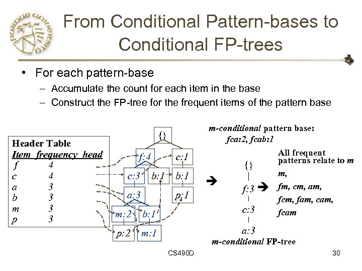 From Conditional Pattern-bases to Conditional FP-trees • For each pattern-base – Accumulate the count for each item in the base – Construct the FP-tree for the frequent items of the pattern base Header Table Item frequency head f 4 c 4 a 3 b 3 m 3 p 3 m-conditional pattern base: fca: 2, fcab: 1 {} f: 4 c: 3 c: 1 b: 1 a: 3 b: 1 p: 1 {} f: 3 m: 2 b: 1 c: 3 p: 2 m: 1 All frequent patterns relate to m m, fm, cm, am, fcm, fam, cam, fcam a: 3 m-conditional FP-tree CS 490 D 30
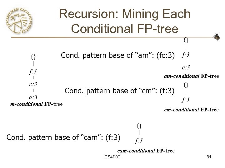 Recursion: Mining Each Conditional FP-tree {} {} Cond. pattern base of “am”: (fc: 3) c: 3 f: 3 c: 3 a: 3 f: 3 am-conditional FP-tree Cond. pattern base of “cm”: (f: 3) {} f: 3 m-conditional FP-tree cm-conditional FP-tree {} Cond. pattern base of “cam”: (f: 3) f: 3 cam-conditional FP-tree CS 490 D 31
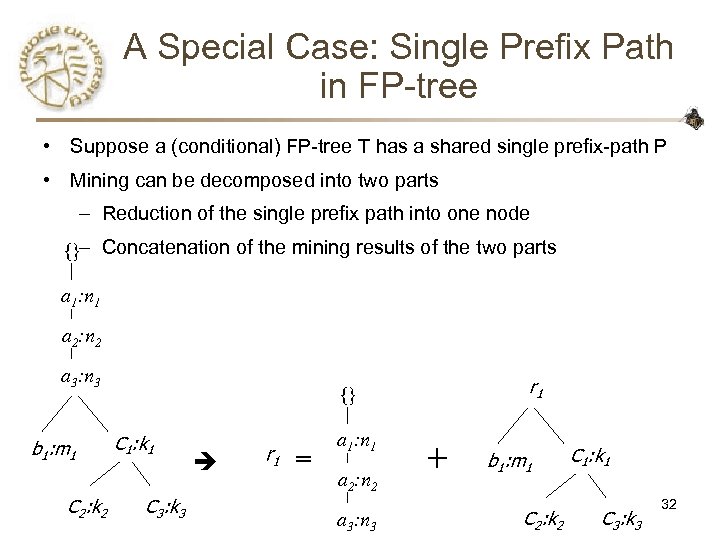 A Special Case: Single Prefix Path in FP-tree • Suppose a (conditional) FP-tree T has a shared single prefix-path P • Mining can be decomposed into two parts – Reduction of the single prefix path into one node {}– Concatenation of the mining results of the two parts a 1: n 1 a 2: n 2 a 3: n 3 b 1: m 1 C 2: k 2 r 1 {} C 1: k 1 C 3: k 3 r 1 = a 1: n 1 a 2: n 2 a 3: n 3 + b 1: m 1 C 2: k 2 C 1: k 1 C 3: k 3 32
 Mining Frequent Patterns With FP-trees • Idea: Frequent pattern growth – Recursively grow frequent patterns by pattern and database partition • Method – For each frequent item, construct its conditional pattern-base, and then its conditional FP-tree – Repeat the process on each newly created conditional FP-tree – Until the resulting FP-tree is empty, or it contains only one path—single path will generate all the combinations of its sub-paths, each of which is a frequent pattern CS 490 D 33
 Scaling FP-growth by DB Projection • FP-tree cannot fit in memory? —DB projection • First partition a database into a set of projected DBs • Then construct and mine FP-tree for each projected DB • Parallel projection vs. Partition projection techniques – Parallel projection is space costly CS 490 D 34
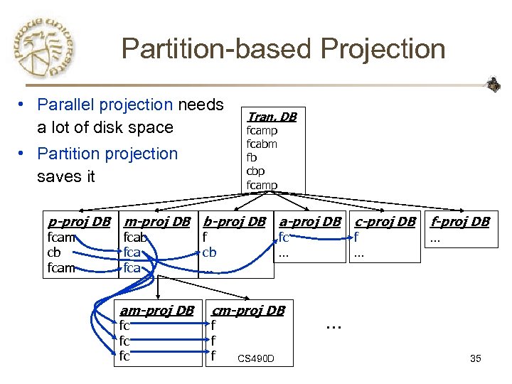 Partition-based Projection • Parallel projection needs a lot of disk space • Partition projection saves it p-proj DB fcam cb fcam Tran. DB fcamp fcabm fb cbp fcamp m-proj DB b-proj DB fcab fca am-proj DB fc fc fc f cb … a-proj DB fc … cm-proj DB f f f CS 490 D c-proj DB f … f-proj DB … … 35
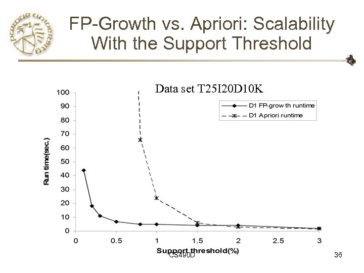 FP-Growth vs. Apriori: Scalability With the Support Threshold Data set T 25 I 20 D 10 K CS 490 D 36
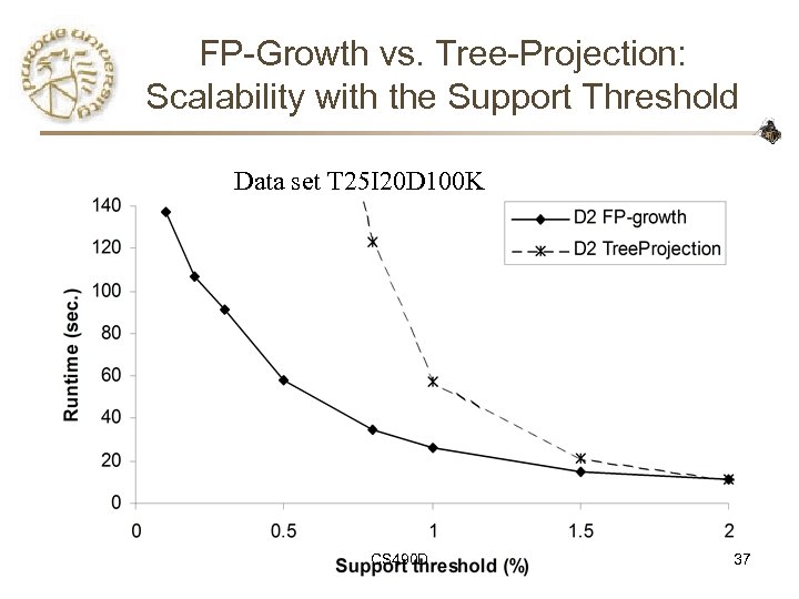 FP-Growth vs. Tree-Projection: Scalability with the Support Threshold Data set T 25 I 20 D 100 K CS 490 D 37
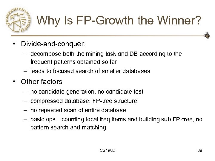 Why Is FP-Growth the Winner? • Divide-and-conquer: – decompose both the mining task and DB according to the frequent patterns obtained so far – leads to focused search of smaller databases • Other factors – no candidate generation, no candidate test – compressed database: FP-tree structure – no repeated scan of entire database – basic ops—counting local freq items and building sub FP-tree, no pattern search and matching CS 490 D 38
 Implications of the Methodology • Mining closed frequent itemsets and max-patterns – CLOSET (DMKD’ 00) • Mining sequential patterns – Free. Span (KDD’ 00), Prefix. Span (ICDE’ 01) • Constraint-based mining of frequent patterns – Convertible constraints (KDD’ 00, ICDE’ 01) • Computing iceberg data cubes with complex measures – H-tree and H-cubing algorithm (SIGMOD’ 01) CS 490 D 39
 Max-patterns • Frequent pattern {a 1, …, a 100} (1001) + (1002) + … + (110000) = 2100 -1 = 1. 27*1030 frequent sub-patterns! • Max-pattern: frequent patterns without proper frequent super pattern – BCDE, ACD are max-patterns Tid 10 – BCD is not a max-pattern 20 Min_sup=2 30 CS 490 D Items A, B, C, D, E, A, C, D, F 40
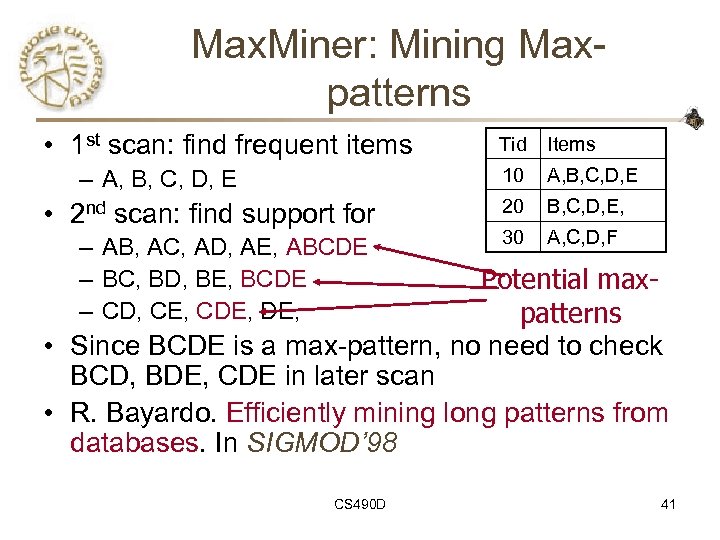 Max. Miner: Mining Maxpatterns • 1 st scan: find frequent items • 2 nd scan: find support for – AB, AC, AD, AE, ABCDE – BC, BD, BE, BCDE – CD, CE, CDE, Items 10 – A, B, C, D, E Tid A, B, C, D, E 20 B, C, D, E, 30 A, C, D, F Potential maxpatterns • Since BCDE is a max-pattern, no need to check BCD, BDE, CDE in later scan • R. Bayardo. Efficiently mining long patterns from databases. In SIGMOD’ 98 CS 490 D 41
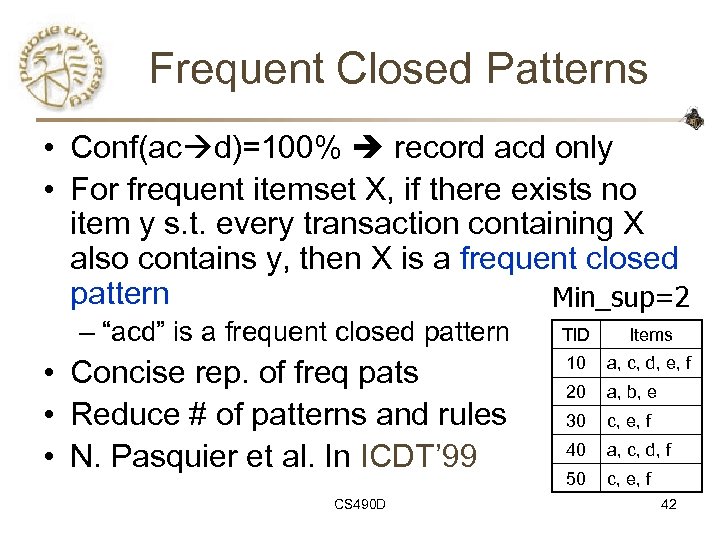 Frequent Closed Patterns • Conf(ac d)=100% record acd only • For frequent itemset X, if there exists no item y s. t. every transaction containing X also contains y, then X is a frequent closed pattern Min_sup=2 – “acd” is a frequent closed pattern TID Items • Concise rep. of freq pats • Reduce # of patterns and rules • N. Pasquier et al. In ICDT’ 99 10 a, c, d, e, f 20 a, b, e 30 c, e, f 40 a, c, d, f 50 c, e, f CS 490 D 42
 Mining Frequent Closed Patterns: CLOSET • Flist: list of all frequent items in support ascending order Min_sup=2 – Flist: d-a-f-e-c • Divide search space – Patterns having d but no a, etc. • Find frequent closed pattern recursively TID 10 20 30 40 50 Items a, c, d, e, f a, b, e c, e, f a, c, d, f c, e, f – Every transaction having d also has cfad is a frequent closed pattern • J. Pei, J. Han & R. Mao. CLOSET: An Efficient Algorithm for Mining Frequent Closed Itemsets", DMKD'00. CS 490 D 43
 Mining Frequent Closed Patterns: CHARM • Use vertical data format: t(AB)={T 1, T 12, …} • Derive closed pattern based on vertical intersections – t(X)=t(Y): X and Y always happen together – t(X) t(Y): transaction having X always has Y • Use diffset to accelerate mining – Only keep track of difference of tids – t(X)={T 1, T 2, T 3}, t(Xy )={T 1, T 3} – Diffset(Xy, X)={T 2} • M. Zaki. CHARM: An Efficient Algorithm for Closed Association Rule Mining, CS-TR 99 -10, Rensselaer Polytechnic Institute • M. Zaki, Fast Vertical Mining Using Diffsets, TR 01 -1, Department of Computer Science, Rensselaer Polytechnic Institute CS 490 D 44
 Visualization of Association Rules: Pane Graph CS 490 D 45
 Visualization of Association Rules: Rule Graph CS 490 D 46
 Mining Association Rules in Large Databases • Association rule mining • Algorithms for scalable mining of (single-dimensional Boolean) association rules in transactional databases • Mining various kinds of association/correlation rules • Constraint-based association mining • Sequential pattern mining • Applications/extensions of frequent pattern mining • Summary CS 490 D 47
 Mining Various Kinds of Rules or Regularities • Multi-level, quantitative association rules, correlation and causality, ratio rules, sequential patterns, emerging patterns, temporal associations, partial periodicity • Classification, clustering, iceberg cubes, etc. CS 490 D 48
 Multiple-level Association Rules • Items often form hierarchy • Flexible support settings: Items at the lower level are expected to have lower support. • Transaction database can be encoded based on dimensions and levels • explore shared multi-level mining reduced support uniform support Level 1 min_sup = 5% Level 2 min_sup = 5% Milk [support = 10%] 2% Milk [support = 6%] Skim Milk [support = 4%] Level 1 min_sup = 5% Level 2 min_sup = 3% 49
 ML/MD Associations with Flexible Support Constraints • Why flexible support constraints? – Real life occurrence frequencies vary greatly • Diamond, watch, pens in a shopping basket – Uniform support may not be an interesting model • A flexible model – The lower-level, the more dimension combination, and the long pattern length, usually the smaller support – General rules should be easy to specify and understand – Special items and special group of items may be specified individually and have higher priority CS 490 D 50
 Multi-dimensional Association • Single-dimensional rules: buys(X, “milk”) buys(X, “bread”) • Multi-dimensional rules: 2 dimensions or predicates – Inter-dimension assoc. rules (no repeated predicates) age(X, ” 19 -25”) occupation(X, “student”) buys(X, “coke”) – hybrid-dimension assoc. rules (repeated predicates) age(X, ” 19 -25”) buys(X, “popcorn”) buys(X, “coke”) • Categorical Attributes – finite number of possible values, no ordering among values • Quantitative Attributes – numeric, implicit ordering among values CS 490 D 51
 Multi-level Association: Redundancy Filtering • Some rules may be redundant due to “ancestor” relationships between items. • Example – milk wheat bread [support = 8%, confidence = 70%] – 2% milk wheat bread [support = 2%, confidence = 72%] • We say the first rule is an ancestor of the second rule. • A rule is redundant if its support is close to the “expected” value, based on the rule’s ancestor. CS 490 D 52
 Multi-Level Mining: Progressive Deepening • A top-down, progressive deepening approach: – First mine high-level frequent items: milk (15%), bread (10%) – Then mine their lower-level “weaker” frequent itemsets: 2% milk (5%), wheat bread (4%) • Different min_support threshold across multilevels lead to different algorithms: – If adopting the same min_support across multi-levels then toss t if any of t’s ancestors is infrequent. – If adopting reduced min_support at lower levels then examine only those descendents whose ancestor’s support is frequent/non-negligible. CS 490 D 53
 Techniques for Mining MD Associations • Search for frequent k-predicate set: – Example: {age, occupation, buys} is a 3 -predicate set – Techniques can be categorized by how age are treated 1. Using static discretization of quantitative attributes – Quantitative attributes are statically discretized by using predefined concept hierarchies 2. Quantitative association rules – Quantitative attributes are dynamically discretized into “bins”based on the distribution of the data 3. Distance-based association rules – This is a dynamic discretization process that considers the distance between data points CS 490 D 54
 CS 490 D: Introduction to Data Mining Prof. Chris Clifton February 6, 2004 Association Rules CS 490 D
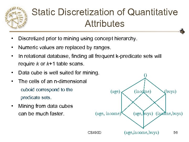 Static Discretization of Quantitative Attributes • Discretized prior to mining using concept hierarchy. • Numeric values are replaced by ranges. • In relational database, finding all frequent k-predicate sets will require k or k+1 table scans. • Data cube is well suited for mining. () • The cells of an n-dimensional cuboid correspond to the (age) (income) (buys) predicate sets. • Mining from data cubes can be much faster. (age, income) CS 490 D (age, buys) (income, buys) (age, income, buys) 56
 Quantitative Association Rules • Numeric attributes are dynamically discretized – Such that the confidence or compactness of the rules mined is maximized • 2 -D quantitative association rules: Aquan 1 Aquan 2 Acat • Cluster “adjacent” association rules to form general rules using a 2 -D grid • Example age(X, ” 30 -34”) income(X, ” 24 K 48 K”) buys(X, ”high resolution TV”) CS 490 D 57
 Mining Distance-based Association Rules • Binning methods do not capture the semantics of interval data • Distance-based partitioning, more meaningful discretization considering: – density/number of points in an interval – “closeness” of points in an interval CS 490 D 58
![Interestingness Measure: Correlations (Lift) • play basketball eat cereal [40%, 66. 7%] is misleading Interestingness Measure: Correlations (Lift) • play basketball eat cereal [40%, 66. 7%] is misleading](https://present5.com/presentation/f67f8f7ed2abb99390d8ed7d63210f22/image-59.jpg) Interestingness Measure: Correlations (Lift) • play basketball eat cereal [40%, 66. 7%] is misleading – The overall percentage of students eating cereal is 75% which is higher than 66. 7%. • play basketball not eat cereal [20%, 33. 3%] is more accurate, although with lower support and confidence • Measure of dependent/correlated events: lift Basketbal Not basketball l Sum (row) Cereal 2000 1750 3750 Not cereal 1000 250 1250 Sum(col. ) 3000 2000 5000 CS 490 D 59
Interestingness Measure: Correlations (Lift) • play basketball eat cereal [40%, 66. 7%] is misleading – The overall percentage of students eating cereal is 75% which is higher than 66. 7%. • play basketball not eat cereal [20%, 33. 3%] is more accurate, although with lower support and confidence • Measure of dependent/correlated events: lift Basketbal Not basketball l Sum (row) Cereal 2000 1750 3750 Not cereal 1000 250 1250 Sum(col. ) 3000 2000 5000 CS 490 D 59
 Mining Association Rules in Large Databases • Association rule mining • Algorithms for scalable mining of (single-dimensional Boolean) association rules in transactional databases • Mining various kinds of association/correlation rules • Constraint-based association mining • Sequential pattern mining • Applications/extensions of frequent pattern mining • Summary CS 490 D 60
 Constraint-based Data Mining • Finding all the patterns in a database autonomously? — unrealistic! – The patterns could be too many but not focused! • Data mining should be an interactive process – User directs what to be mined using a data mining query language (or a graphical user interface) • Constraint-based mining – User flexibility: provides constraints on what to be mined – System optimization: explores such constraints for efficient mining—constraint-based mining CS 490 D 61
 Constraints in Data Mining • Knowledge type constraint: – classification, association, etc. • Data constraint — using SQL-like queries – find product pairs sold together in stores in Vancouver in Dec. ’ 00 • Dimension/level constraint – in relevance to region, price, brand, customer category • Rule (or pattern) constraint – small sales (price < $10) triggers big sales (sum > $200) • Interestingness constraint – strong rules: min_support 3%, min_confidence 60% CS 490 D 62
 Constrained Mining vs. Constraint. Based Search • Constrained mining vs. constraint-based search/reasoning – Both are aimed at reducing search space – Finding all patterns satisfying constraints vs. finding some (or one) answer in constraint-based search in AI – Constraint-pushing vs. heuristic search – It is an interesting research problem on how to integrate them • Constrained mining vs. query processing in DBMS – Database query processing requires to find all – Constrained pattern mining shares a similar philosophy as pushing selections deeply in query processing CS 490 D 63
 Constrained Frequent Pattern Mining: A Mining Query Optimization Problem • Given a frequent pattern mining query with a set of constraints C, the algorithm should be – sound: it only finds frequent sets that satisfy the given constraints C – complete: all frequent sets satisfying the given constraints C are found • A naïve solution – First find all frequent sets, and then test them for constraint satisfaction • More efficient approaches: – Analyze the properties of constraints comprehensively – Push them as deeply as possible inside the frequent pattern computation. CS 490 D 64
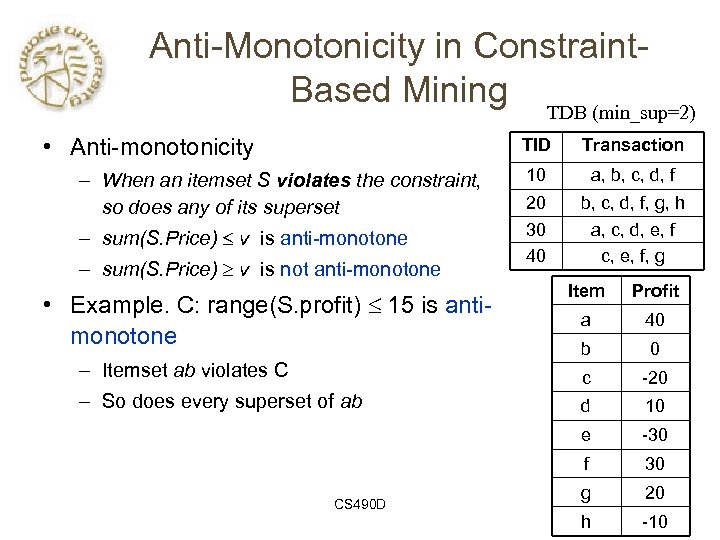 Anti-Monotonicity in Constraint. Based Mining TDB (min_sup=2) • Anti-monotonicity TID – When an itemset S violates the constraint, so does any of its superset – sum(S. Price) v is anti-monotone – sum(S. Price) v is not anti-monotone Transaction 10 a, b, c, d, f 20 30 40 b, c, d, f, g, h a, c, d, e, f c, e, f, g CS 490 D 40 b 0 -20 d 10 -30 f – So does every superset of ab a e – Itemset ab violates C Profit c • Example. C: range(S. profit) 15 is antimonotone Item 30 g 20 h -10
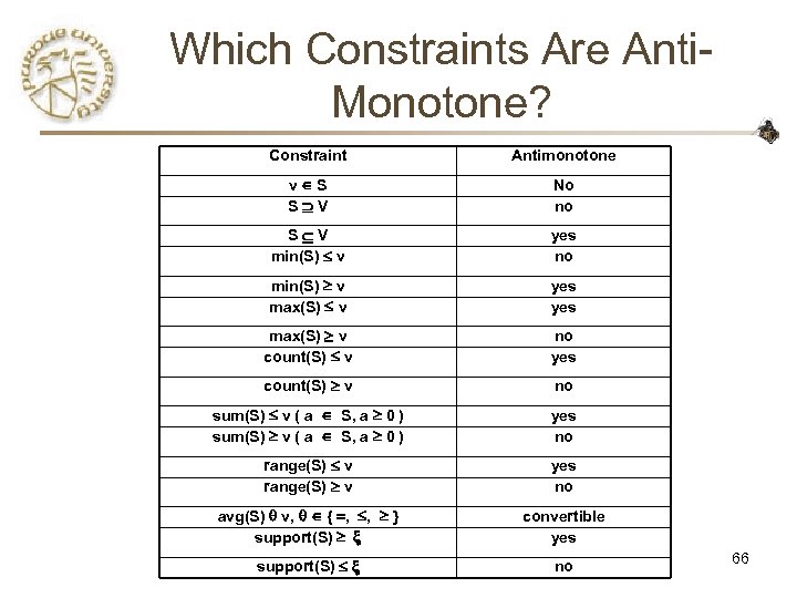 Which Constraints Are Anti. Monotone? Constraint Antimonotone v S S V No no S V min(S) v yes no min(S) v max(S) v yes max(S) v count(S) v no yes count(S) v no sum(S) v ( a S, a 0 ) yes no range(S) v yes no avg(S) v, { , , } support(S) convertible yes support(S) no 66
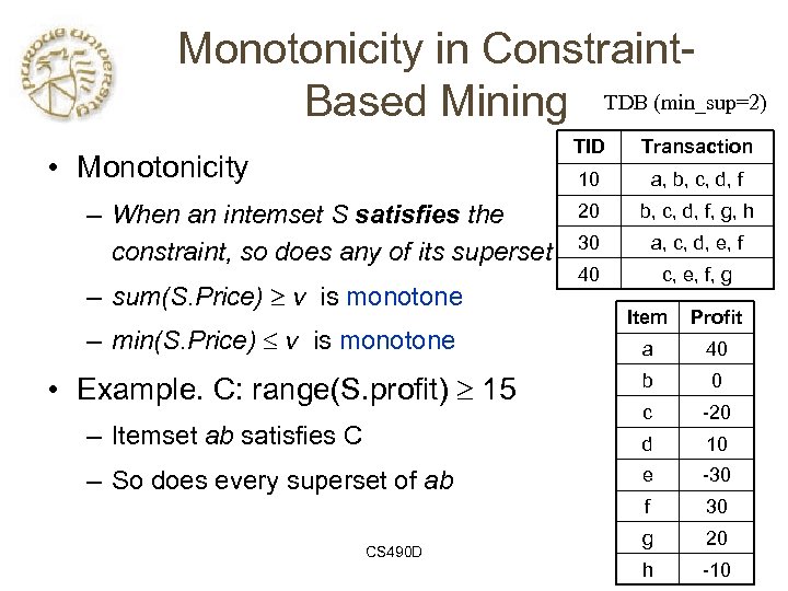 Monotonicity in Constraint. Based Mining TDB (min_sup=2) TID 10 • Monotonicity – When an intemset S satisfies the constraint, so does any of its superset – sum(S. Price) v is monotone Transaction a, b, c, d, f 20 b, c, d, f, g, h 30 a, c, d, e, f 40 c, e, f, g Item Profit a 40 b 0 – Itemset ab satisfies C c -20 d 10 – So does every superset of ab e -30 f 30 g 20 h -10 – min(S. Price) v is monotone • Example. C: range(S. profit) 15 CS 490 D
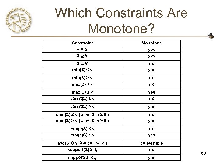 Which Constraints Are Monotone? Constraint v S S V Monotone yes S V min(S) v no yes min(S) v max(S) v no no max(S) v count(S) v yes no count(S) v yes sum(S) v ( a S, a 0 ) no yes range(S) v no yes avg(S) v, { , , } support(S) convertible no support(S) yes 68
 Succinctness • Succinctness: – Given A 1, the set of items satisfying a succinctness constraint C, then any set S satisfying C is based on A 1 , i. e. , S contains a subset belonging to A 1 – Idea: Without looking at the transaction database, whether an itemset S satisfies constraint C can be determined based on the selection of items – min(S. Price) v is succinct – sum(S. Price) v is not succinct • Optimization: If C is succinct, C is pre-counting pushable CS 490 D 69
 Which Constraints Are Succinct? Constraint v S S V Succinct yes S V min(S) v yes min(S) v max(S) v yes max(S) v count(S) v yes weakly count(S) v weakly sum(S) v ( a S, a 0 ) no no range(S) v no no avg(S) v, { , , } support(S) no no support(S) no 70
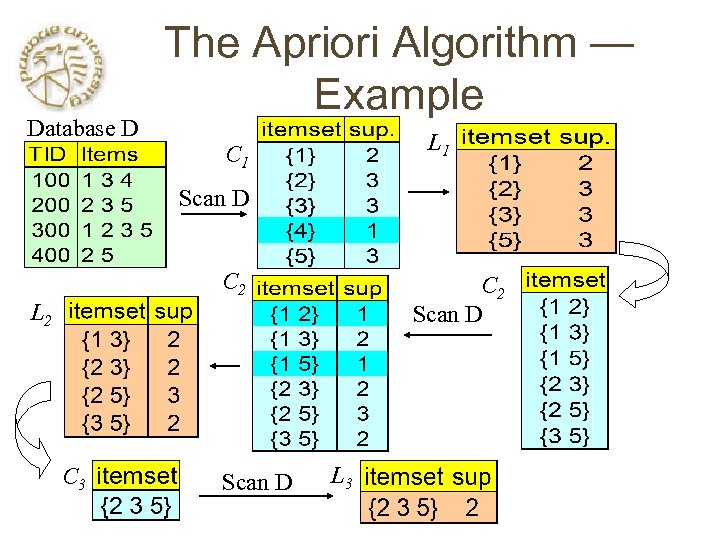 Database D The Apriori Algorithm — Example L 1 C 1 Scan D C 2 Scan D L 2 C 3 Scan D L 3
 Database D Naïve Algorithm: Apriori + Constraint L 1 C 1 Scan D C 2 Scan D L 2 C 3 Scan D L 3 Constraint: Sum{S. price < 5}
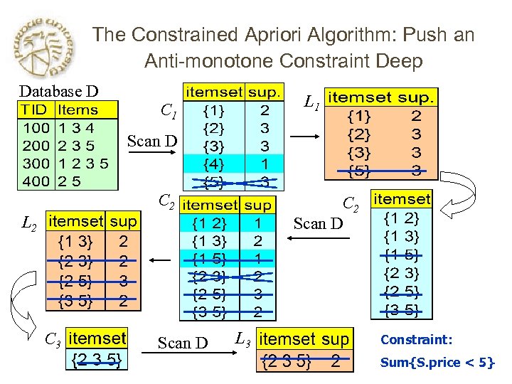 The Constrained Apriori Algorithm: Push an Anti-monotone Constraint Deep Database D L 1 C 1 Scan D C 2 Scan D L 2 C 3 Scan D L 3 Constraint: Sum{S. price < 5}
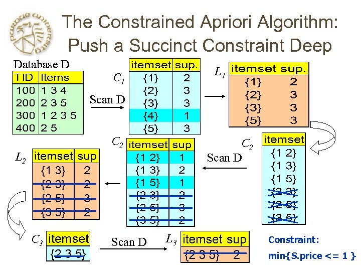 The Constrained Apriori Algorithm: Push a Succinct Constraint Deep Database D L 1 C 1 Scan D C 2 Scan D L 2 C 3 Scan D L 3 Constraint: min{S. price <= 1 }
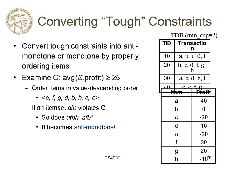 Converting “Tough” Constraints TDB (min_sup=2) • Convert tough constraints into antimonotone or monotone by properly ordering items TID • Examine C: avg(S. profit) 25 30 – Order items in value-descending order •
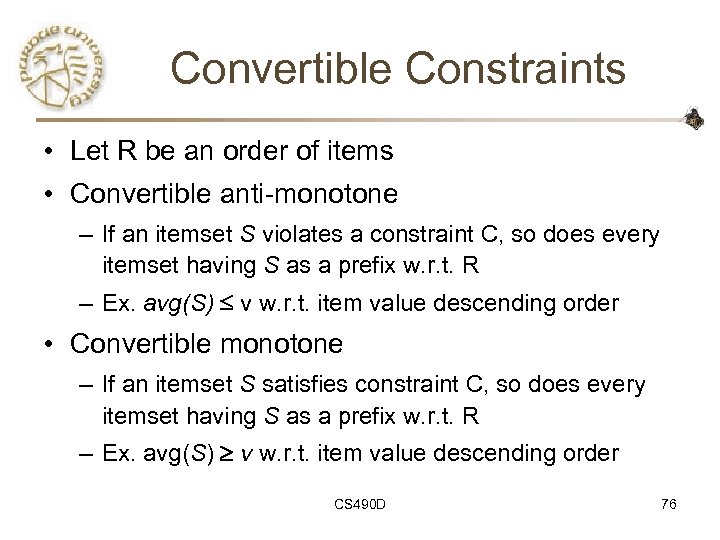 Convertible Constraints • Let R be an order of items • Convertible anti-monotone – If an itemset S violates a constraint C, so does every itemset having S as a prefix w. r. t. R – Ex. avg(S) v w. r. t. item value descending order • Convertible monotone – If an itemset S satisfies constraint C, so does every itemset having S as a prefix w. r. t. R – Ex. avg(S) v w. r. t. item value descending order CS 490 D 76
 Strongly Convertible Constraints • avg(X) 25 is convertible anti-monotone w. r. t. item value descending order R:
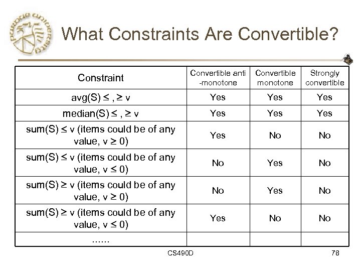 What Constraints Are Convertible? Constraint Convertible anti -monotone Convertible monotone Strongly convertible avg(S) , v Yes Yes median(S) , v Yes Yes sum(S) v (items could be of any value, v 0) Yes No No sum(S) v (items could be of any value, v 0) No Yes No sum(S) v (items could be of any value, v 0) Yes No No …… CS 490 D 78
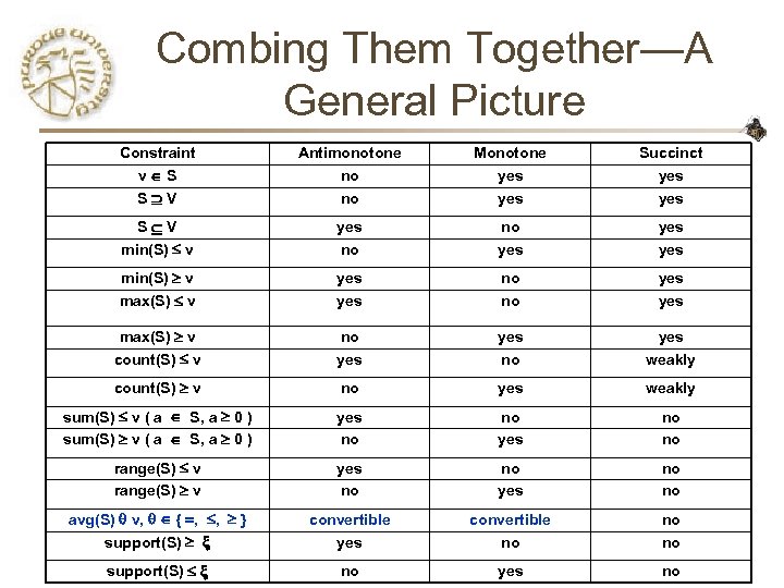 Combing Them Together—A General Picture Constraint v S S V Antimonotone no no Monotone yes Succinct yes S V min(S) v yes no no yes yes min(S) v max(S) v yes no no yes max(S) v count(S) v no yes weakly count(S) v no yes weakly sum(S) v ( a S, a 0 ) yes no no range(S) v yes no no avg(S) v, { , , } support(S) convertible yes convertible no no no support(S) no yes no
 Classification of Constraints Monotone Antimonotone Succinct Strongly convertible Convertible anti-monotone Convertible monotone Inconvertible CS 490 D 80
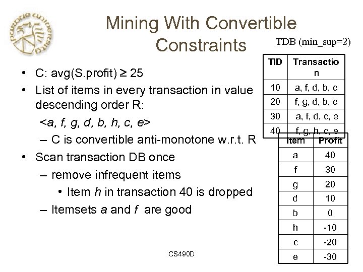 Mining With Convertible TDB (min_sup=2) Constraints • C: avg(S. profit) 25 • List of items in every transaction in value descending order R:
 Can Apriori Handle Convertible Constraint? • A convertible, not monotone nor antimonotone nor succinct constraint cannot be pushed deep into the an Apriori mining algorithm – Within the level wise framework, no direct pruning based on the constraint can be made – Itemset df violates constraint C: avg(X)>=25 – Since adf satisfies C, Apriori needs df to assemble adf, df cannot be pruned • But it can be pushed into frequentpattern growth framework! CS 490 D Item Value a 40 b 0 c -20 d 10 e -30 f 30 g 20 h -10 82
 Mining With Convertible Constraints Item Value • C: avg(X)>=25, min_sup=2 a 40 • List items in every transaction in value descending order R:
 Handling Multiple Constraints • Different constraints may require different or even conflicting item-ordering • If there exists an order R s. t. both C 1 and C 2 are convertible w. r. t. R, then there is no conflict between the two convertible constraints • If there exists conflict on order of items – Try to satisfy one constraint first – Then using the order for the other constraint to mine frequent itemsets in the corresponding projected database CS 490 D 84
 Mining Association Rules in Large Databases • Association rule mining • Algorithms for scalable mining of (single-dimensional Boolean) association rules in transactional databases • Mining various kinds of association/correlation rules • Constraint-based association mining • Sequential pattern mining • Applications/extensions of frequent pattern mining • Summary CS 490 D 85
 Sequence Databases and Sequential Pattern Analysis • Transaction databases, time-series databases vs. sequence databases • Frequent patterns vs. (frequent) sequential patterns • Applications of sequential pattern mining – Customer shopping sequences: • First buy computer, then CD-ROM, and then digital camera, within 3 months. – Medical treatment, natural disasters (e. g. , earthquakes), science & engineering processes, stocks and markets, etc. – Telephone calling patterns, Weblog click streams – DNA sequences and gene structures CS 490 D 86
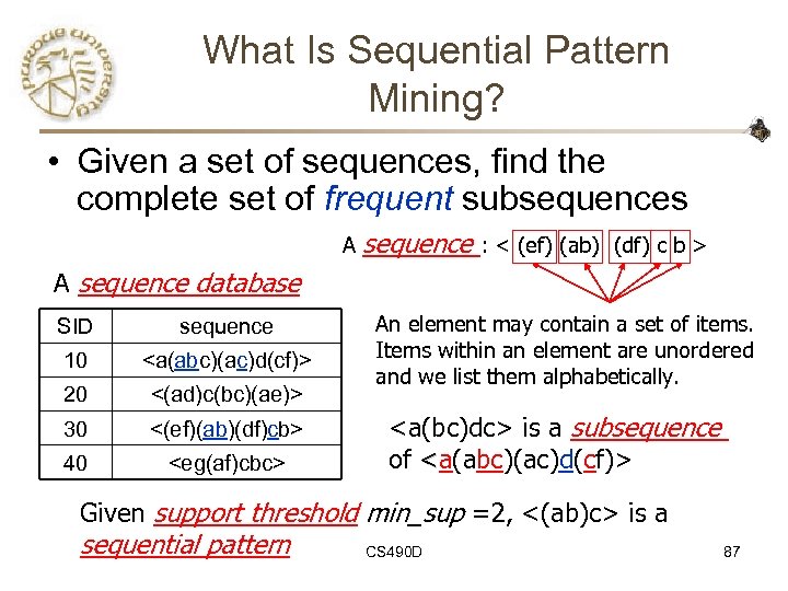 What Is Sequential Pattern Mining? • Given a set of sequences, find the complete set of frequent subsequences A sequence : < (ef) (ab) (df) c b > A sequence database SID sequence 10
 Challenges on Sequential Pattern Mining • A huge number of possible sequential patterns are hidden in databases • A mining algorithm should – find the complete set of patterns, when possible, satisfying the minimum support (frequency) threshold – be highly efficient, scalable, involving only a small number of database scans – be able to incorporate various kinds of user-specific constraints CS 490 D 88
 Studies on Sequential Pattern Mining • Concept introduction and an initial Apriori-like algorithm – R. Agrawal & R. Srikant. “Mining sequential patterns, ” ICDE’ 95 • GSP—An Apriori-based, influential mining method (developed at IBM Almaden) – R. Srikant & R. Agrawal. “Mining sequential patterns: Generalizations and performance improvements, ” EDBT’ 96 • From sequential patterns to episodes (Apriori-like + constraints) – H. Mannila, H. Toivonen & A. I. Verkamo. “Discovery of frequent episodes in event sequences, ” Data Mining and Knowledge Discovery, 1997 • Mining sequential patterns with constraints – M. N. Garofalakis, R. Rastogi, K. Shim: SPIRIT: Sequential Pattern Mining with Regular Expression Constraints. VLDB 1999 CS 490 D 89
 A Basic Property of Sequential Patterns: Apriori • A basic property: Apriori (Agrawal & Sirkant’ 94) – If a sequence S is not frequent – Then none of the super-sequences of S is frequent – E. g,
 GSP—A Generalized Sequential Pattern Mining Algorithm • GSP (Generalized Sequential Pattern) mining algorithm – proposed by Agrawal and Srikant, EDBT’ 96 • Outline of the method – Initially, every item in DB is a candidate of length-1 – for each level (i. e. , sequences of length-k) do • scan database to collect support count for each candidate sequence • generate candidate length-(k+1) sequences from length-k frequent sequences using Apriori – repeat until no frequent sequence or no candidate can be found • Major strength: Candidate pruning by Apriori CS 490 D 91
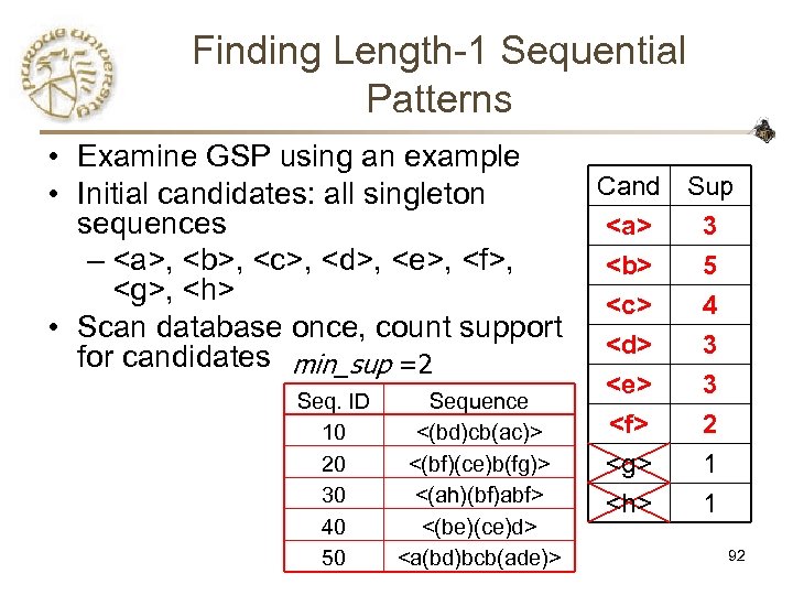 Finding Length-1 Sequential Patterns • Examine GSP using an example • Initial candidates: all singleton sequences – , ,
 Generating Length-2 Candidates
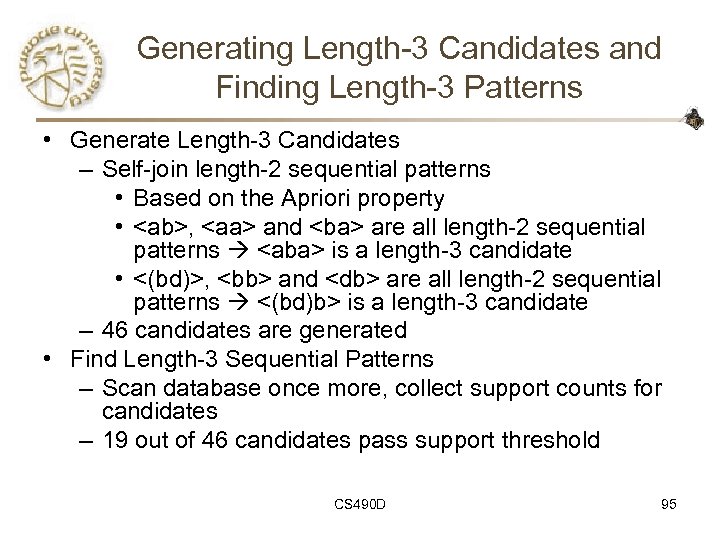 Generating Length-3 Candidates and Finding Length-3 Patterns • Generate Length-3 Candidates – Self-join length-2 sequential patterns • Based on the Apriori property •
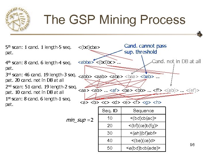 The GSP Mining Process 5 th scan: 1 cand. 1 length-5 seq. pat. Cand. cannot pass sup. threshold <(bd)cba> Cand. not in DB at all 4 th scan: 8 cand. 6 length-4 seq.
 Bottlenecks of GSP • A huge set of candidates could be generated – 1, 000 frequent length-1 sequences generate length-2 candidates! • Multiple scans of database in mining • Real challenge: mining long sequential patterns – An exponential number of short candidates – A length-100 sequential pattern needs 1030 candidate sequences! CS 490 D 98
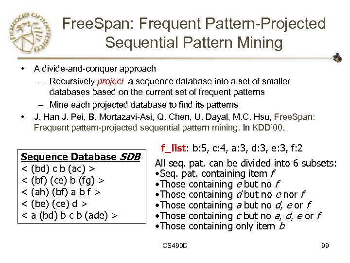 Free. Span: Frequent Pattern-Projected Sequential Pattern Mining • • A divide-and-conquer approach – Recursively project a sequence database into a set of smaller databases based on the current set of frequent patterns – Mine each projected database to find its patterns J. Han J. Pei, B. Mortazavi-Asi, Q. Chen, U. Dayal, M. C. Hsu, Free. Span: Frequent pattern-projected sequential pattern mining. In KDD’ 00. Sequence Database SDB < (bd) c b (ac) > < (bf) (ce) b (fg) > < (ah) (bf) a b f > < (be) (ce) d > < a (bd) b c b (ade) > f_list: b: 5, c: 4, a: 3, d: 3, e: 3, f: 2 All seq. pat. can be divided into 6 subsets: • Seq. pat. containing item f • Those containing e but no f • Those containing d but no e nor f • Those containing a but no d, e or f • Those containing c but no a, d, e or f • Those containing only item b CS 490 D 99
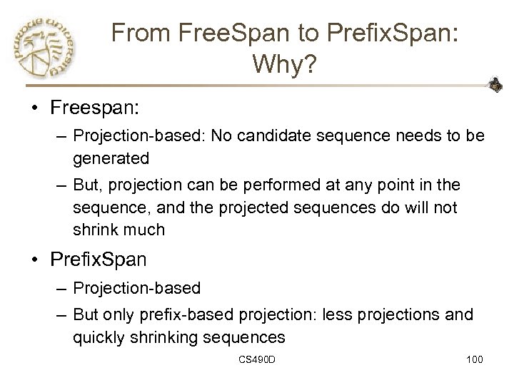 From Free. Span to Prefix. Span: Why? • Freespan: – Projection-based: No candidate sequence needs to be generated – But, projection can be performed at any point in the sequence, and the projected sequences do will not shrink much • Prefix. Span – Projection-based – But only prefix-based projection: less projections and quickly shrinking sequences CS 490 D 100
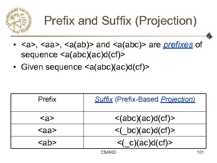 Prefix and Suffix (Projection) • ,
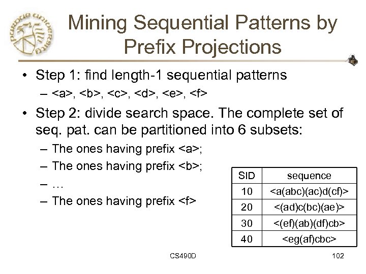 Mining Sequential Patterns by Prefix Projections • Step 1: find length-1 sequential patterns – , ,
 Finding Seq. Patterns with Prefix • Only need to consider projections w. r. t. – -projected database: <(abc)(ac)d(cf)>, <(_d)c(bc)(ae)>, <(_b)(df)cb>, <(_f)cbc> • Find all the length-2 seq. pat. Having prefix :
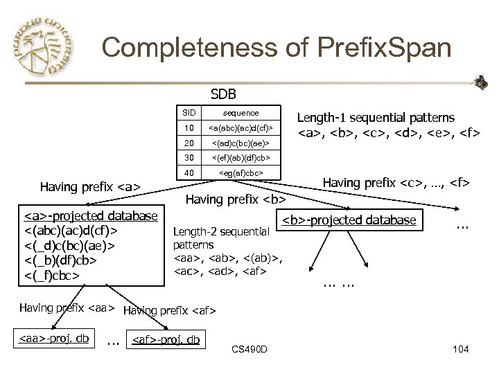 Completeness of Prefix. Span SDB SID 10 <(ad)c(bc)(ae)> 30 <(ef)(ab)(df)cb> 40 -projected database <(abc)(ac)d(cf)> <(_d)c(bc)(ae)> <(_b)(df)cb> <(_f)cbc>
 Efficiency of Prefix. Span • No candidate sequence needs to be generated • Projected databases keep shrinking • Major cost of Prefix. Span: constructing projected databases – Can be improved by bi-level projections CS 490 D 105
 Optimization Techniques in Prefix. Span • Physical projection vs. pseudo-projection – Pseudo-projection may reduce the effort of projection when the projected database fits in main memory • Parallel projection vs. partition projection – Partition projection may avoid the blowup of disk space CS 490 D 106
 Speed-up by Pseudoprojection • Major cost of Prefix. Span: projection – Postfixes of sequences often appear repeatedly in recursive projected databases • When (projected) database can be held in main memory, use pointers to form projections – Pointer to the sequence – Offset of the postfix s=
 Pseudo-Projection vs. Physical Projection • Pseudo-projection avoids physically copying postfixes – Efficient in running time and space when database can be held in main memory • However, it is not efficient when database cannot fit in main memory – Disk-based random accessing is very costly • Suggested Approach: – Integration of physical and pseudo-projection – Swapping to pseudo-projection when the data set fits in memory CS 490 D 108
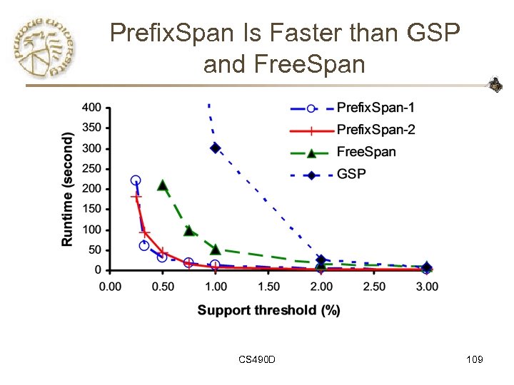 Prefix. Span Is Faster than GSP and Free. Span CS 490 D 109
 Effect of Pseudo-Projection CS 490 D 110
 Mining Association Rules in Large Databases • Association rule mining • Algorithms for scalable mining of (single-dimensional Boolean) association rules in transactional databases • Mining various kinds of association/correlation rules • Constraint-based association mining • Sequential pattern mining • Applications/extensions of frequent pattern mining • Summary CS 490 D 111
 Associative Classification • Mine association possible rules (PR) in form of condset c – Condset: a set of attribute-value pairs – C: class label • Build Classifier – Organize rules according to decreasing precedence based on confidence and support • B. Liu, W. Hsu & Y. Ma. Integrating classification and association rule mining. In KDD’ 98 CS 490 D 112
 Spatial and Multi-Media Association: A Progressive Refinement Method • Why progressive refinement? – Mining operator can be expensive or cheap, fine or rough – Trade speed with quality: step-by-step refinement. • Superset coverage property: – Preserve all the positive answers—allow a positive false test but not a false negative test. • Two- or multi-step mining: – First apply rough/cheap operator (superset coverage) – Then apply expensive algorithm on a substantially reduced candidate set (Koperski & Han, SSD’ 95). CS 490 D 116
 Progressive Refinement Mining of Spatial Associations • Hierarchy of spatial relationship: – “g_close_to”: near_by, touch, intersect, contain, etc. – First search for rough relationship and then refine it. • Two-step mining of spatial association: – Step 1: rough spatial computation (as a filter) • Using MBR or R-tree for rough estimation. – Step 2: Detailed spatial algorithm (as refinement) • Apply only to those objects which have passed the rough spatial association test (no less than min_support)
 Mining Multimedia Associations Correlations with color, spatial relationships, etc. From coarse to Fine Resolution mining CS 490 D 118
 Further Evolution of Prefix. Span • Closed- and max- sequential patterns – Finding only the most meaningful (longest) sequential patterns • Constraint-based sequential pattern growth – Adding user-specific constraints • From sequential patterns to structured patterns – Beyond sequential patterns, mining structured patterns in XML documents CS 490 D 119
 Closed- and Max- Sequential Patterns • A closed- sequential pattern is a frequent sequence s where there is no proper super-sequence of s sharing the same support count with s • A max- sequential pattern is a sequential pattern p s. t. any proper super-pattern of p is not frequent • Benefit of the notion of closed sequential patterns – {, }, with min_sup = 1 – There are 2100 sequential patterns, but only 2 are closed • Similar benefits for the notion of max- sequential-patterns CS 490 D 120
 Methods for Mining Closedand Max- Sequential Patterns • Prefix. Span or Free. Span can be viewed as projectionguided depth-first search • For mining max- sequential patterns, any sequence which does not contain anything beyond the already discovered ones will be removed from the projected DB – {, }, with min_sup = 1 – If we have found a max-sequential pattern , nothing will be projected in any projected DB • Similar ideas can be applied for mining closedsequential-patterns CS 490 D 121
 Constraint-Based Sequential Pattern Mining • Constraint-based sequential pattern mining – Constraints: User-specified, for focused mining of desired patterns – How to explore efficient mining with constraints? — Optimization • Classification of constraints – Anti-monotone: E. g. , value_sum(S) < 150, min(S) > 10 – Monotone: E. g. , count (S) > 5, S {PC, digital_camera} – Succinct: E. g. , length(S) 10, S {Pentium, MS/Office, MS/Money} – Convertible: E. g. , value_avg(S) < 25, profit_sum (S) > 160, max(S)/avg(S) < 2, median(S) – min(S) > 5 – Inconvertible: E. g. , avg(S) – median(S) = 0 CS 490 D 122
 Sequential Pattern Growth for Constraint-Based Mining • Efficient mining with convertible constraints – Not solvable by candidate generation-and-test methodology – Easily push-able into the sequential pattern growth framework • Example: push avg(S) < 25 in frequent pattern growth – project items in value (price/profit depending on mining semantics) ascending/descending order for sequential pattern growth – Grow each pattern by sequential pattern growth – If avg(current_pattern) 25, toss the current_pattern • Why? —future growths always make it bigger • But why not candidate generation? —no structure or ordering in growth CS 490 D 123
 From Sequential Patterns to Structured Patterns • Sets, sequences, trees and other structures – Transaction DB: Sets of items • {{i 1, i 2, …, im}, …} – Seq. DB: Sequences of sets: • {<{i 1, i 2}, …, {im, in, ik}>, …} – Sets of Sequences: • {{, …,
 Mining Association Rules in Large Databases • Association rule mining • Algorithms for scalable mining of (single-dimensional Boolean) association rules in transactional databases • Mining various kinds of association/correlation rules • Constraint-based association mining • Sequential pattern mining • Applications/extensions of frequent pattern mining • Summary CS 490 D 125
 Frequent-Pattern Mining: Achievements • Frequent pattern mining—an important task in data mining • Frequent pattern mining methodology – Candidate generation & test vs. projection-based (frequent-pattern growth) – Vertical vs. horizontal format – Various optimization methods: database partition, scan reduction, hash tree, sampling, border computation, clustering, etc. • Related frequent-pattern mining algorithm: scope extension – Mining closed frequent itemsets and max-patterns (e. g. , Max. Miner, CLOSET, CHARM, etc. ) – Mining multi-level, multi-dimensional frequent patterns with flexible support constraints – Constraint pushing for mining optimization – From frequent patterns to correlation and causality CS 490 D 126
 Frequent-Pattern Mining: Applications • Related problems which need frequent pattern mining – Association-based classification – Iceberg cube computation – Database compression by fascicles and frequent patterns – Mining sequential patterns (GSP, Prefix. Span, SPADE, etc. ) – Mining partial periodicity, cyclic associations, etc. – Mining frequent structures, trends, etc. • Typical application examples – Market-basket analysis, Weblog analysis, DNA mining, etc. CS 490 D 127
 Frequent-Pattern Mining: Research Problems • Multi-dimensional gradient analysis: patterns regarding changes and differences – Not just counts—other measures, e. g. , avg(profit) • Mining top-k frequent patterns without support constraint • Mining fault-tolerant associations – “ 3 out of 4 courses excellent” leads to A in data mining • Fascicles and database compression by frequent pattern mining • Partial periodic patterns • DNA sequence analysis and pattern classification CS 490 D 128
 References: Frequent-pattern Mining Methods • R. Agarwal, C. Aggarwal, and V. V. V. Prasad. A tree projection algorithm for generation of frequent itemsets. Journal of Parallel and Distributed Computing, 2000. • R. Agrawal, T. Imielinski, and A. Swami. Mining association rules between sets of items in large databases. SIGMOD'93, 207 -216, Washington, D. C. • R. Agrawal and R. Srikant. Fast algorithms for mining association rules. VLDB'94 487 -499, Santiago, Chile. • J. Han, J. Pei, and Y. Yin: “Mining frequent patterns without candidate generation”. In Proc. ACM-SIGMOD’ 2000, pp. 1 -12, Dallas, TX, May 2000. • H. Mannila, H. Toivonen, and A. I. Verkamo. Efficient algorithms for discovering association rules. KDD'94, 181 -192, Seattle, WA, July 1994. CS 490 D 129
 References: Frequent-pattern Mining Methods • A. Savasere, E. Omiecinski, and S. Navathe. An efficient algorithm for mining association rules in large databases. VLDB'95, 432 -443, Zurich, Switzerland. • C. Silverstein, S. Brin, R. Motwani, and J. Ullman. Scalable techniques for mining causal structures. VLDB'98, 594 -605, New York, NY. • R. Srikant and R. Agrawal. Mining generalized association rules. VLDB'95, 407 -419, Zurich, Switzerland, Sept. 1995. • R. Srikant and R. Agrawal. Mining quantitative association rules in large relational tables. SIGMOD'96, 1 -12, Montreal, Canada. • H. Toivonen. Sampling large databases for association rules. VLDB'96, 134 -145, Bombay, India, Sept. 1996. • M. J. Zaki, S. Parthasarathy, M. Ogihara, and W. Li. New algorithms for fast discovery of association rules. KDD’ 97. August 1997. CS 490 D 130
 References: Frequent-pattern Mining (Performance Improvements) • S. Brin, R. Motwani, J. D. Ullman, and S. Tsur. Dynamic itemset counting and implication rules for market basket analysis. SIGMOD'97, Tucson, Arizona, May 1997. • D. W. Cheung, J. Han, V. Ng, and C. Y. Wong. Maintenance of discovered association rules in large databases: An incremental updating technique. ICDE'96, New Orleans, LA. • T. Fukuda, Y. Morimoto, S. Morishita, and T. Tokuyama. Data mining using two-dimensional optimized association rules: Scheme, algorithms, and visualization. SIGMOD'96, Montreal, Canada. • E. -H. Han, G. Karypis, and V. Kumar. Scalable parallel data mining for association rules. SIGMOD'97, Tucson, Arizona. • J. S. Park, M. S. Chen, and P. S. Yu. An effective hash-based algorithm for mining association rules. SIGMOD'95, San Jose, CA, May 1995. CS 490 D 131
 References: Frequent-pattern Mining (Performance Improvements) • G. Piatetsky-Shapiro. Discovery, analysis, and presentation of strong rules. In G. Piatetsky-Shapiro and W. J. Frawley, Knowledge Discovery in Databases, . AAAI/MIT Press, 1991. • J. S. Park, M. S. Chen, and P. S. Yu. An effective hash-based algorithm for mining association rules. SIGMOD'95, San Jose, CA. • S. Sarawagi, S. Thomas, and R. Agrawal. Integrating association rule mining with relational database systems: Alternatives and implications. SIGMOD'98, Seattle, WA. • K. Yoda, T. Fukuda, Y. Morimoto, S. Morishita, and T. Tokuyama. Computing optimized rectilinear regions for association rules. KDD'97, Newport Beach, CA, Aug. 1997. • M. J. Zaki, S. Parthasarathy, M. Ogihara, and W. Li. Parallel algorithm for discovery of association rules. Data Mining and Knowledge Discovery, 1: 343 -374, 1997. CS 490 D 132
 References: Frequent-pattern Mining (Multilevel, correlation, ratio rules, etc. ) • S. Brin, R. Motwani, and C. Silverstein. Beyond market basket: Generalizing association rules to correlations. SIGMOD'97, 265 -276, Tucson, Arizona. • J. Han and Y. Fu. Discovery of multiple-level association rules from large databases. VLDB'95, 420 -431, Zurich, Switzerland. • M. Klemettinen, H. Mannila, P. Ronkainen, H. Toivonen, and A. I. Verkamo. Finding interesting rules from large sets of discovered association rules. CIKM'94, 401 -408, Gaithersburg, Maryland. • F. Korn, A. Labrinidis, Y. Kotidis, and C. Faloutsos. Ratio rules: A new paradigm for fast, quantifiable data mining. VLDB'98, 582 -593, New York, NY • • B. Lent, A. Swami, and J. Widom. Clustering association rules. ICDE'97, 220 -231, Birmingham, England. • • R. J. Miller and Y. Yang. Association rules over interval data. SIGMOD'97, 452 -461, Tucson, Arizona. • D. Tsur, J. D. Ullman, S. Abitboul, C. Clifton, R. Motwani, and S. Nestorov. Query flocks: A generalization of association-rule mining. SIGMOD'98, 1 -12, Seattle, Washington. • J. Pei, A. K. H. Tung, J. Han. Fault-Tolerant Frequent Pattern Mining: Problems and Challenges. SIGMOD DMKD’ 01, Santa Barbara, CA. R. Meo, G. Psaila, and S. Ceri. A new SQL-like operator for mining association rules. VLDB'96, 122 -133, Bombay, India. A. Savasere, E. Omiecinski, and S. Navathe. Mining for strong negative associations in a large database of customer transactions. ICDE'98, 494 -502, Orlando, FL, Feb. 1998. CS 490 D 133
 References: Mining Max-patterns and Closed itemsets • R. J. Bayardo. Efficiently mining long patterns from databases. SIGMOD'98, 85 -93, Seattle, Washington. • J. Pei, J. Han, and R. Mao, "CLOSET: An Efficient Algorithm for Mining Frequent Closed Itemsets", Proc. 2000 ACM-SIGMOD Int. Workshop on Data Mining and Knowledge Discovery (DMKD'00), Dallas, TX, May 2000. • N. Pasquier, Y. Bastide, R. Taouil, and L. Lakhal. Discovering frequent closed itemsets for association rules. ICDT'99, 398 -416, Jerusalem, Israel, Jan. 1999. • M. Zaki. Generating Non-Redundant Association Rules. KDD'00. Boston, MA. Aug. 2000 • M. Zaki. CHARM: An Efficient Algorithm for Closed Association Rule Mining, SIAM’ 02 CS 490 D 134
 References: Constraint-base Frequent-pattern Mining • G. Grahne, L. Lakshmanan, and X. Wang. Efficient mining of constrained correlated sets. ICDE'00, 512 -521, San Diego, CA, Feb. 2000. • Y. Fu and J. Han. Meta-rule-guided mining of association rules in relational databases. KDOOD'95, 39 -46, Singapore, Dec. 1995. • J. Han, L. V. S. Lakshmanan, and R. T. Ng, "Constraint-Based, Multidimensional Data Mining", COMPUTER (special issues on Data Mining), 32(8): 46 -50, 1999. • L. V. S. Lakshmanan, R. Ng, J. Han and A. Pang, "Optimization of Constrained Frequent Set Queries with 2 Variable Constraints", SIGMOD’ 99 • R. Ng, L. V. S. Lakshmanan, J. Han & A. Pang. “Exploratory mining and pruning optimizations of constrained association rules. ” SIGMOD’ 98 • J. Pei, J. Han, and L. V. S. Lakshmanan, "Mining Frequent Itemsets with Convertible Constraints", Proc. 2001 Int. Conf. on Data Engineering (ICDE'01), April 2001. • J. Pei and J. Han "Can We Push More Constraints into Frequent Pattern Mining? ", Proc. 2000 Int. Conf. on Knowledge Discovery and Data Mining (KDD'00), Boston, MA, August 2000. • R. Srikant, Q. Vu, and R. Agrawal. Mining association rules with item constraints. KDD'97, 67 -73, Newport Beach, California CS 490 D 135
 References: Sequential Pattern Mining Methods • R. Agrawal and R. Srikant. Mining sequential patterns. ICDE'95, 314, Taipei, Taiwan. • R. Srikant and R. Agrawal. Mining sequential patterns: Generalizations and performance improvements. EDBT’ 96. • J. Han, J. Pei, B. Mortazavi-Asl, Q. Chen, U. Dayal, M. -C. Hsu, "Free. Span: Frequent Pattern-Projected Sequential Pattern Mining", Proc. 2000 Int. Conf. on Knowledge Discovery and Data Mining (KDD'00), Boston, MA, August 2000. • H. Mannila, H Toivonen, and A. I. Verkamo. Discovery of frequent episodes in event sequences. Data Mining and Knowledge Discovery, 1: 259 -289, 1997. CS 490 D 136
 References: Sequential Pattern Mining Methods • J. Pei, J. Han, H. Pinto, Q. Chen, U. Dayal, and M. -C. Hsu, "Prefix. Span: Mining Sequential Patterns Efficiently by Prefix-Projected Pattern Growth", Proc. 2001 Int. Conf. on Data Engineering (ICDE'01), Heidelberg, Germany, April 2001. • B. Ozden, S. Ramaswamy, and A. Silberschatz. Cyclic association rules. ICDE'98, 412 -421, Orlando, FL. • S. Ramaswamy, S. Mahajan, and A. Silberschatz. On the discovery of interesting patterns in association rules. VLDB'98, 368 -379, New York, NY. • M. J. Zaki. Efficient enumeration of frequent sequences. CIKM’ 98. Novermber 1998. • M. N. Garofalakis, R. Rastogi, K. Shim: SPIRIT: Sequential Pattern Mining with Regular Expression Constraints. VLDB 1999: 223 -234, Edinburgh, Scotland. CS 490 D 137
 References: Frequent-pattern Mining in Spatial, Multimedia, Text & Web Databases • K. Koperski, J. Han, and G. B. Marchisio, "Mining Spatial and Image Data through Progressive Refinement Methods", Revue internationale de gomatique (European Journal of GIS and Spatial Analysis), 9(4): 425 -440, 1999. • A. K. H. Tung, H. Lu, J. Han, and L. Feng, "Breaking the Barrier of Transactions: Mining Inter-Transaction Association Rules", Proc. 1999 Int. Conf. on Knowledge Discovery and Data Mining (KDD'99), San Diego, CA, Aug. 1999, pp. 297 -301. • J. Han, G. Dong and Y. Yin, "Efficient Mining of Partial Periodic Patterns in Time Series Database", Proc. 1999 Int. Conf. on Data Engineering (ICDE'99), Sydney, Australia, March 1999, pp. 106 -115 • H. Lu, L. Feng, and J. Han, "Beyond Intra-Transaction Association Analysis: Mining Multi-Dimensional Inter. Transaction Association Rules", ACM Transactions on Information Systems (TOIS’ 00), 18(4): 423 -454, 2000. • O. R. Zaiane, M. Xin, J. Han, "Discovering Web Access Patterns and Trends by Applying OLAP and Data Mining Technology on Web Logs, " Proc. Advances in Digital Librar ies Conf. (ADL'98), Santa Barbara, CA, April 1998, pp. 19 -29 • O. R. Zaiane, J. Han, and H. Zhu, "Mining Recurrent Items in Multimedia with Progressive Resolution Refinement", ICDE'00, San Diego, CA, Feb. 2000, pp. 461 -470 CS 490 D 138
 References: Frequent-pattern Mining for Classification and Data Cube Computation • K. Beyer and R. Ramakrishnan. Bottom-up computation of sparse and iceberg cubes. SIGMOD'99, 359 -370, Philadelphia, PA, June 1999. • M. Fang, N. Shivakumar, H. Garcia-Molina, R. Motwani, and J. D. Ullman. Computing iceberg queries efficiently. VLDB'98, 299 -310, New York, NY, Aug. 1998. • J. Han, J. Pei, G. Dong, and K. Wang, “Computing Iceberg Data Cubes with Complex Measures”, Proc. ACM-SIGMOD’ 2001, Santa Barbara, CA, May 2001. • M. Kamber, J. Han, and J. Y. Chiang. Metarule-guided mining of multi-dimensional association rules using data cubes. KDD'97, 207 -210, Newport Beach, California. • K. Beyer and R. Ramakrishnan. Bottom-up computation of sparse and iceberg cubes. SIGMOD’ 99 • T. Imielinski, L. Khachiyan, and A. Abdulghani. Cubegrades: Generalizing association rules. Technical Report, Aug. 2000 CS 490 D 139


