CS 490 D Introduction to Data Mining Chris

CS 490 D: Introduction to Data Mining Chris Clifton January 16, 2004 Data Warehousing CS 490 D

Data Warehousing and OLAP Technology for Data Mining • • • What is a data warehouse? A multi-dimensional data model Data warehouse architecture Data warehouse implementation Further development of data cube technology • From data warehousing to data mining CS 490 D 2

What is Data Warehouse? • Defined in many different ways, but not rigorously. – A decision support database that is maintained separately from the organization’s operational database – Support information processing by providing a solid platform of consolidated, historical data for analysis. • “A data warehouse is a subject-oriented, integrated, time-variant, and nonvolatile collection of data in support of management’s decisionmaking process. ”—W. H. Inmon • Data warehousing: – The process of constructing and using data warehouses CS 490 D 3

Data Warehouse—Subject. Oriented • Organized around major subjects, such as customer, product, sales. • Focusing on the modeling and analysis of data for decision makers, not on daily operations or transaction processing. • Provide a simple and concise view around particular subject issues by excluding data that are not useful in the decision support process. CS 490 D 4

Data Warehouse—Integrated • Constructed by integrating multiple, heterogeneous data sources – relational databases, flat files, on-line transaction records • Data cleaning and data integration techniques are applied. – Ensure consistency in naming conventions, encoding structures, attribute measures, etc. among different data sources • E. g. , Hotel price: currency, tax, breakfast covered, etc. – When data is moved to the warehouse, it is converted. CS 490 D 5

Data Warehouse—Time Variant • The time horizon for the data warehouse is significantly longer than that of operational systems. – Operational database: current value data. – Data warehouse data: provide information from a historical perspective (e. g. , past 5 -10 years) • Every key structure in the data warehouse – Contains an element of time, explicitly or implicitly – But the key of operational data may or may not contain “time element”. CS 490 D 6

Data Warehouse—Non-Volatile • A physically separate store of data transformed from the operational environment. • Operational update of data does not occur in the data warehouse environment. – Does not require transaction processing, recovery, and concurrency control mechanisms – Requires only two operations in data accessing: • initial loading of data and access of data. CS 490 D 7

Data Warehouse vs. Heterogeneous DBMS • Traditional heterogeneous DB integration: – Build wrappers/mediators on top of heterogeneous databases – Query driven approach • When a query is posed to a client site, a meta-dictionary is used to translate the query into queries appropriate for individual heterogeneous sites involved, and the results are integrated into a global answer set • Complex information filtering, compete for resources • Data warehouse: update-driven, high performance – Information from heterogeneous sources is integrated in advance and stored in warehouses for direct query and analysis CS 490 D 8

Data Warehouse vs. Operational DBMS • OLTP (on-line transaction processing) – Major task of traditional relational DBMS – Day-to-day operations: purchasing, inventory, banking, manufacturing, payroll, registration, accounting, etc. • OLAP (on-line analytical processing) – Major task of data warehouse system – Data analysis and decision making • Distinct features (OLTP vs. OLAP): – – – User and system orientation: customer vs. market Data contents: current, detailed vs. historical, consolidated Database design: ER + application vs. star + subject View: current, local vs. evolutionary, integrated Access patterns: update vs. read-only but complex queries CS 490 D 9

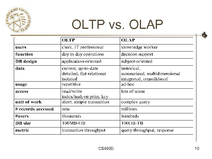OLTP vs. OLAP CS 490 D 10

Why Separate Data Warehouse? • High performance for both systems – DBMS— tuned for OLTP: access methods, indexing, concurrency control, recovery – Warehouse—tuned for OLAP: complex OLAP queries, multidimensional view, consolidation. • Different functions and different data: – missing data: Decision support requires historical data which operational DBs do not typically maintain – data consolidation: DS requires consolidation (aggregation, summarization) of data from heterogeneous sources – data quality: different sources typically use inconsistent data representations, codes and formats which have to be reconciled CS 490 D 11

Data Warehousing and OLAP Technology for Data Mining • • • What is a data warehouse? A multi-dimensional data model Data warehouse architecture Data warehouse implementation Further development of data cube technology • From data warehousing to data mining CS 490 D 12

From Tables and Spreadsheets to Data Cubes • A data warehouse is based on a multidimensional data model which views data in the form of a data cube • A data cube, such as sales, allows data to be modeled and viewed in multiple dimensions – Dimension tables, such as item (item_name, brand, type), or time(day, week, month, quarter, year) – Fact table contains measures (such as dollars_sold) and keys to each of the related dimension tables • In data warehousing literature, an n-D base cube is called a base cuboid. The top most 0 -D cuboid, which holds the highest-level of summarization, is called the apex cuboid. The lattice of cuboids forms a data cube. CS 490 D 13

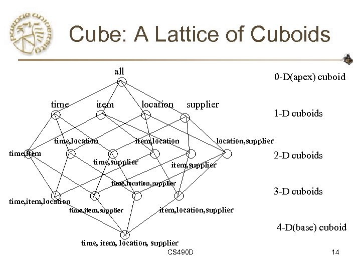Cube: A Lattice of Cuboids all time 0 -D(apex) cuboid item time, location time, item location supplier item, location time, supplier location, supplier item, supplier time, location, supplier time, item, location time, item, supplier 1 -D cuboids 2 -D cuboids 3 -D cuboids item, location, supplier 4 -D(base) cuboid time, item, location, supplier CS 490 D 14

CS 490 D: Introduction to Data Mining Chris Clifton January 21, 2004 Data Warehousing CS 490 D

Conceptual Modeling of Data Warehouses • Modeling data warehouses: dimensions & measures – Star schema: A fact table in the middle connected to a set of dimension tables – Snowflake schema: A refinement of star schema where some dimensional hierarchy is normalized into a set of smaller dimension tables, forming a shape similar to snowflake – Fact constellations: Multiple fact tables share dimension tables, viewed as a collection of stars, therefore called galaxy schema or fact constellation CS 490 D 16

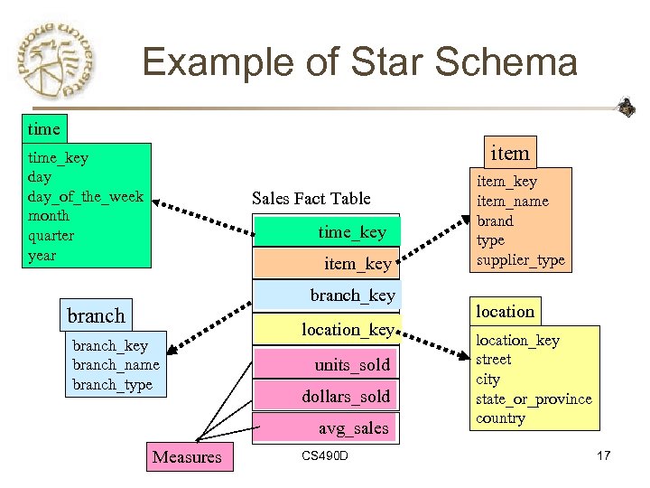Example of Star Schema time item time_key day_of_the_week month quarter year Sales Fact Table time_key item_key branch_key branch_name branch_type location_key units_sold dollars_sold avg_sales Measures CS 490 D item_key item_name brand type supplier_type location_key street city state_or_province country 17

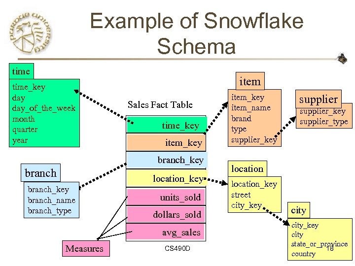Example of Snowflake Schema time_key day_of_the_week month quarter year item Sales Fact Table time_key item_key branch location_key branch_name branch_type units_sold dollars_sold avg_sales Measures CS 490 D item_key item_name brand type supplier_key supplier_type location_key street city_key city state_or_province 18 country

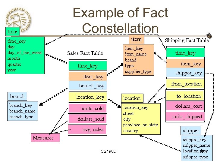Example of Fact Constellation time_key day_of_the_week month quarter year item Sales Fact Table time_key item_key item_name brand type supplier_type location_key branch_name branch_type units_sold dollars_sold avg_sales Measures CS 490 D time_key item_key shipper_key from_location branch_key branch Shipping Fact Table location to_location_key street city province_or_state country dollars_cost units_shipped shipper_key shipper_name location_key 19 shipper_type

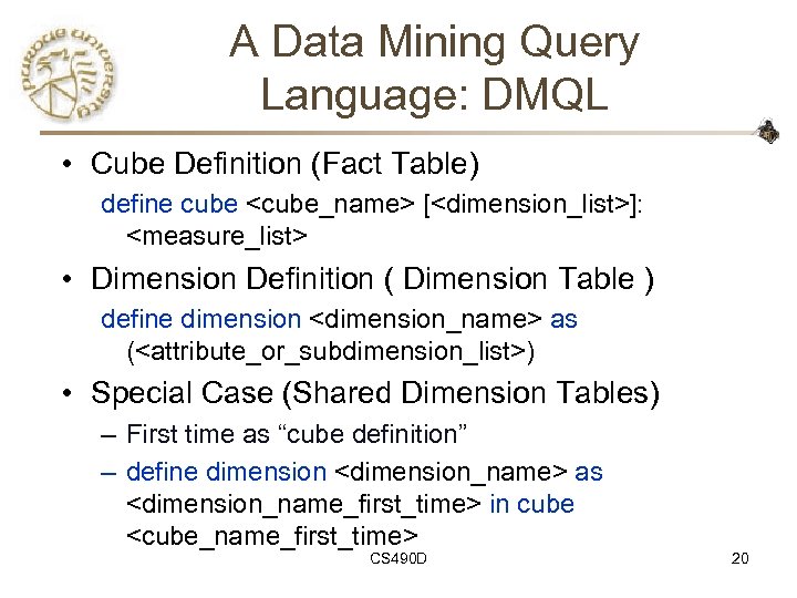A Data Mining Query Language: DMQL • Cube Definition (Fact Table) define cube []: • Dimension Definition ( Dimension Table ) define dimension as () • Special Case (Shared Dimension Tables) – First time as “cube definition” – define dimension as in cube CS 490 D 20

Defining a Star Schema in DMQL define cube sales_star [time, item, branch, location]: dollars_sold = sum(sales_in_dollars), avg_sales = avg(sales_in_dollars), units_sold = count(*) define dimension time as (time_key, day_of_week, month, quarter, year) define dimension item as (item_key, item_name, brand, type, supplier_type) define dimension branch as (branch_key, branch_name, branch_type) define dimension location as (location_key, street, city, province_or_state, country) CS 490 D 21

Defining a Snowflake Schema in DMQL define cube sales_snowflake [time, item, branch, location]: dollars_sold = sum(sales_in_dollars), avg_sales = avg(sales_in_dollars), units_sold = count(*) define dimension time as (time_key, day_of_week, month, quarter, year) define dimension item as (item_key, item_name, brand, type, supplier(supplier_key, supplier_type)) define dimension branch as (branch_key, branch_name, branch_type) define dimension location as (location_key, street, city(city_key, province_or_state, country)) CS 490 D 22

Defining a Fact Constellation in DMQL define cube sales [time, item, branch, location]: dollars_sold = sum(sales_in_dollars), avg_sales = avg(sales_in_dollars), units_sold = count(*) define dimension time as (time_key, day_of_week, month, quarter, year) define dimension item as (item_key, item_name, brand, type, supplier_type) define dimension branch as (branch_key, branch_name, branch_type) define dimension location as (location_key, street, city, province_or_state, country) define cube shipping [time, item, shipper, from_location, to_location]: dollar_cost = sum(cost_in_dollars), unit_shipped = count(*) define dimension time as time in cube sales define dimension item as item in cube sales define dimension shipper as (shipper_key, shipper_name, location as location in cube sales, shipper_type) define dimension from_location as location in cube sales define dimension to_location as location in cube sales CS 490 D 23

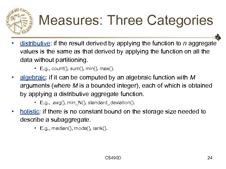Measures: Three Categories • distributive: if the result derived by applying the function to n aggregate values is the same as that derived by applying the function on all the data without partitioning. • E. g. , count(), sum(), min(), max(). • algebraic: if it can be computed by an algebraic function with M arguments (where M is a bounded integer), each of which is obtained by applying a distributive aggregate function. • E. g. , avg(), min_N(), standard_deviation(). • holistic: if there is no constant bound on the storage size needed to describe a subaggregate. • E. g. , median(), mode(), rank(). CS 490 D 24

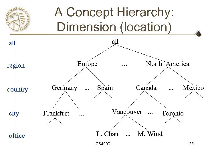A Concept Hierarchy: Dimension (location) all Europe region country city office Germany Frankfurt . . . Spain North_America Canada Vancouver. . . L. Chan CS 490 D . . . Mexico Toronto M. Wind 25

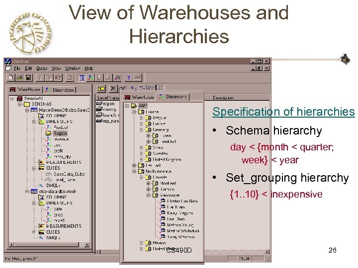View of Warehouses and Hierarchies Specification of hierarchies • Schema hierarchy day < {month < quarter; week} < year • Set_grouping hierarchy {1. . 10} < inexpensive CS 490 D 26

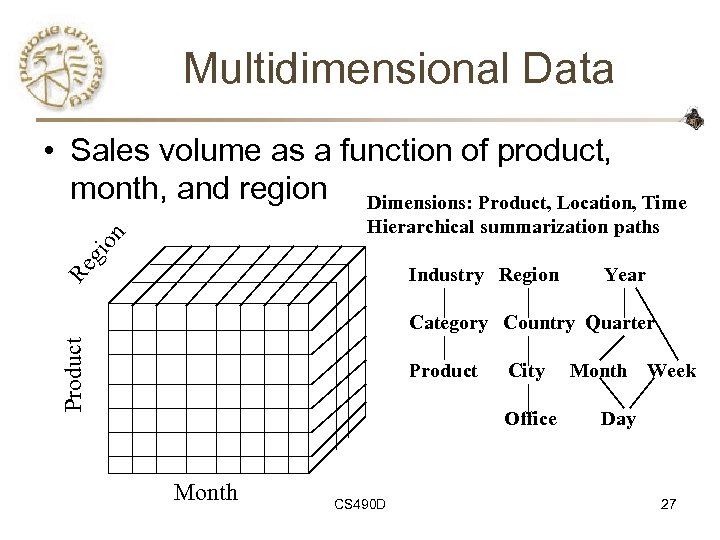Multidimensional Data • Sales volume as a function of product, month, and region Dimensions: Product, Location, Time gi on Hierarchical summarization paths Re Industry Region Year Product Category Country Quarter Product City Office Month CS 490 D Month Week Day 27

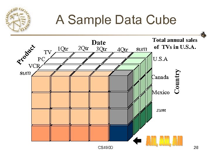2 Qtr 3 Qtr od TV PC VCR sum 1 Qtr Date 4 Qtr Total annual sales sum of TVs in U. S. A. Pr U. S. A Canada Mexico Country uc t A Sample Data Cube sum CS 490 D 28

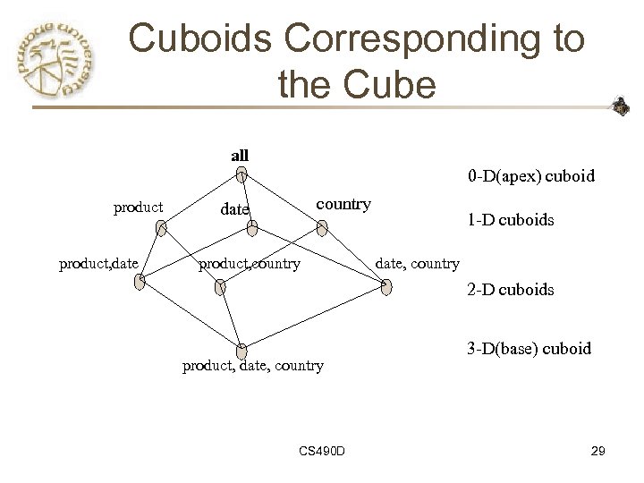Cuboids Corresponding to the Cube all 0 -D(apex) cuboid product, date country date product, country 1 -D cuboids date, country 2 -D cuboids product, date, country CS 490 D 3 -D(base) cuboid 29

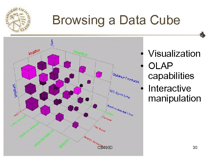Browsing a Data Cube • Visualization • OLAP capabilities • Interactive manipulation CS 490 D 30

Typical OLAP Operations • Roll up (drill-up): summarize data – by climbing up hierarchy or by dimension reduction • Drill down (roll down): reverse of roll-up – from higher level summary to lower level summary or detailed data, or introducing new dimensions • Slice and dice: – project and select • Pivot (rotate): – reorient the cube, visualization, 3 D to series of 2 D planes. • Other operations – drill across: involving (across) more than one fact table – drill through: through the bottom level of the cube to its back-end relational tables (using SQL) CS 490 D 31

Data Warehousing and OLAP Technology for Data Mining • • • What is a data warehouse? A multi-dimensional data model Data warehouse architecture Data warehouse implementation Further development of data cube technology • From data warehousing to data mining CS 490 D 40

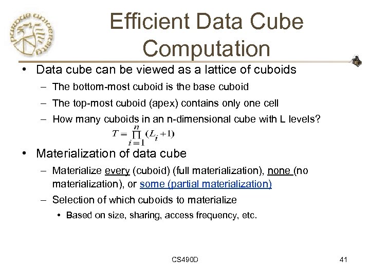Efficient Data Cube Computation • Data cube can be viewed as a lattice of cuboids – The bottom-most cuboid is the base cuboid – The top-most cuboid (apex) contains only one cell – How many cuboids in an n-dimensional cube with L levels? • Materialization of data cube – Materialize every (cuboid) (full materialization), none (no materialization), or some (partial materialization) – Selection of which cuboids to materialize • Based on size, sharing, access frequency, etc. CS 490 D 41

Cube Operation • Cube definition and computation in DMQL define cube sales[item, city, year]: sum(sales_in_dollars) compute cube sales • Transform it into a SQL-like language (with a new operator cube by, introduced by Gray et al. ’ 96) () SELECT item, city, year, SUM (amount) FROM SALES (city) CUBE BY item, city, year (item) (year) • Need compute the following Group-Bys (date, product, customer), (city, item) (city, year) (item, year) (date, product), (date, customer), (product, customer), (date), (product), (customer) () (city, item, year) CS 490 D 42

Cube Computation: ROLAPBased Method • Efficient cube computation methods – – ROLAP-based cubing algorithms (Agarwal et al’ 96) Array-based cubing algorithm (Zhao et al’ 97) Bottom-up computation method (Beyer & Ramarkrishnan’ 99) H-cubing technique (Han, Pei, Dong & Wang: SIGMOD’ 01) • ROLAP-based cubing algorithms – Sorting, hashing, and grouping operations are applied to the dimension attributes in order to reorder and cluster related tuples – Grouping is performed on some sub-aggregates as a “partial grouping step” – Aggregates may be computed from previously computed aggregates, rather than from the base fact table CS 490 D 43

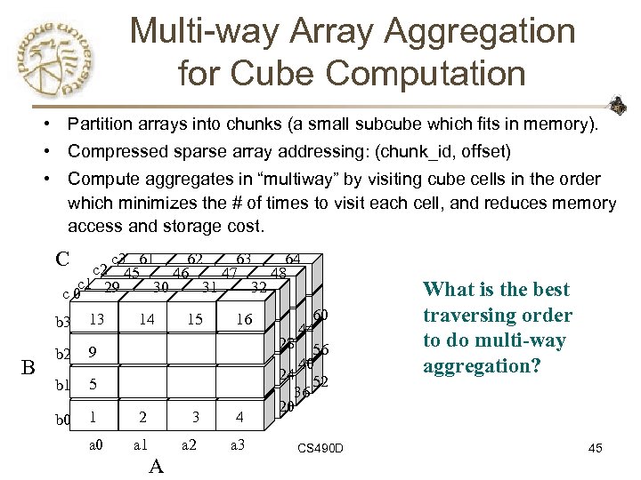Multi-way Array Aggregation for Cube Computation • Partition arrays into chunks (a small subcube which fits in memory). • Compressed sparse array addressing: (chunk_id, offset) • Compute aggregates in “multiway” by visiting cube cells in the order which minimizes the # of times to visit each cell, and reduces memory access and storage cost. C c 3 61 62 63 64 c 2 45 46 47 48 c 1 29 30 31 32 c 0 b 3 B B 13 b 2 9 b 1 5 b 0 14 15 16 1 2 3 4 a 0 a 1 a 2 a 3 A 60 44 28 56 40 24 52 36 20 CS 490 D What is the best traversing order to do multi-way aggregation? 45

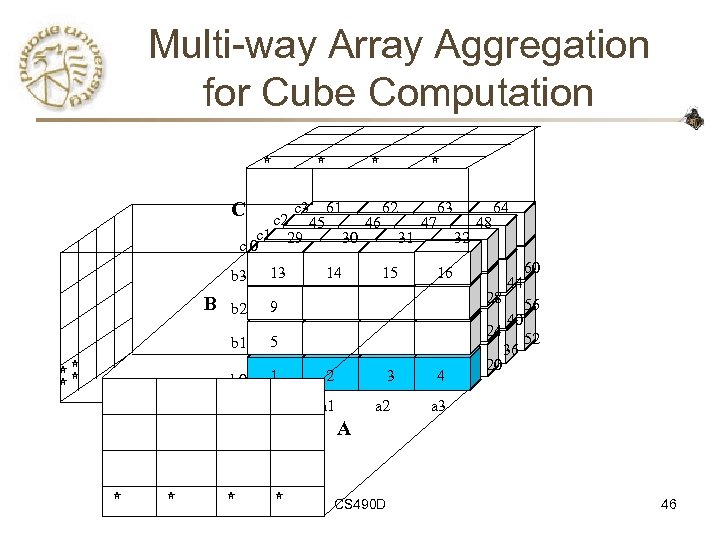Multi-way Array Aggregation for Cube Computation C c 3 61 62 63 64 c 2 45 46 47 48 c 1 29 30 31 32 c 0 b 3 B b 2 B 13 14 15 16 28 9 24 b 1 5 b 0 1 2 3 4 a 0 a 1 a 2 44 40 60 56 52 a 3 20 36 A CS 490 D 46

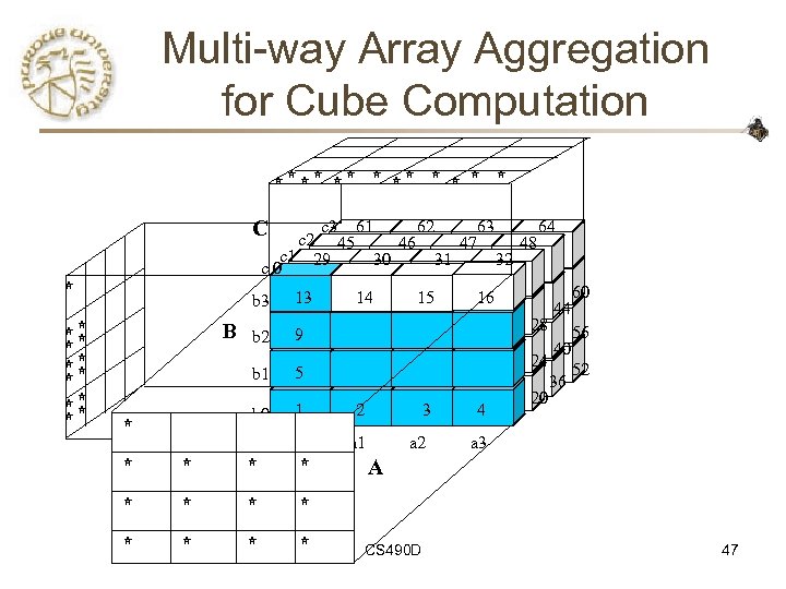Multi-way Array Aggregation for Cube Computation C c 3 61 62 63 64 c 2 45 46 47 48 c 1 29 30 31 32 c 0 b 3 B b 2 B 13 14 15 16 28 9 24 b 1 5 b 0 1 2 3 4 a 0 a 1 a 2 44 40 60 56 52 a 3 20 36 A CS 490 D 47

Multi-Way Array Aggregation for Cube Computation (Cont. ) • Method: the planes should be sorted and computed according to their size in ascending order. – See the details of Example 2. 12 (pp. 75 -78) – Idea: keep the smallest plane in the main memory, fetch and compute only one chunk at a time for the largest plane • Limitation of the method: computing well only for a small number of dimensions – If there a large number of dimensions, “bottom-up computation” and iceberg cube computation methods can be explored CS 490 D 48

Data Warehousing and OLAP Technology for Data Mining • • • What is a data warehouse? A multi-dimensional data model Data warehouse architecture Data warehouse implementation Further development of data cube technology • From data warehousing to data mining CS 490 D 75

Data Warehouse Usage • Three kinds of data warehouse applications – Information processing • supports querying, basic statistical analysis, and reporting using crosstabs, tables, charts and graphs – Analytical processing • multidimensional analysis of data warehouse data • supports basic OLAP operations, slice-dice, drilling, pivoting – Data mining • knowledge discovery from hidden patterns • supports associations, constructing analytical models, performing classification and prediction, and presenting the mining results using visualization tools. • Differences among the three tasks CS 490 D 76

From On-Line Analytical Processing to On Line Analytical Mining (OLAM) • Why online analytical mining? – High quality of data in data warehouses • DW contains integrated, consistent, cleaned data – Available information processing structure surrounding data warehouses • ODBC, OLEDB, Web accessing, service facilities, reporting and OLAP tools – OLAP-based exploratory data analysis • mining with drilling, dicing, pivoting, etc. – On-line selection of data mining functions • integration and swapping of multiple mining functions, algorithms, and tasks. CS 490 D 77

Discovery-Driven Exploration of Data Cubes • Hypothesis-driven – exploration by user, huge search space • Discovery-driven (Sarawagi, et al. ’ 98) – Effective navigation of large OLAP data cubes – pre-compute measures indicating exceptions, guide user in the data analysis, at all levels of aggregation – Exception: significantly different from the value anticipated, based on a statistical model – Visual cues such as background color are used to reflect the degree of exception of each cell CS 490 D 79

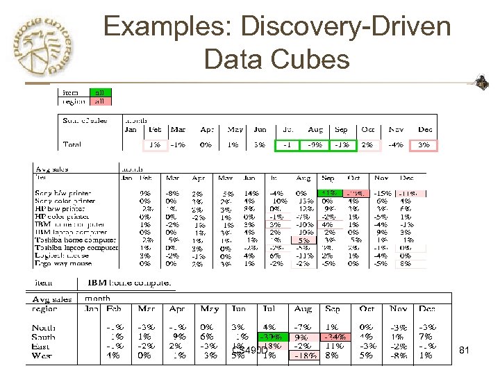Examples: Discovery-Driven Data Cubes CS 490 D 81

Summary • Data warehouse • A multi-dimensional model of a data warehouse – Star schema, snowflake schema, fact constellations – A data cube consists of dimensions & measures • OLAP operations: drilling, rolling, slicing, dicing and pivoting • OLAP servers: ROLAP, MOLAP, HOLAP • Efficient computation of data cubes – Partial vs. full vs. no materialization – Multiway array aggregation – Bitmap index and join index implementations • Further development of data cube technology – Discovery-drive and multi-feature cubes – From OLAP to OLAM (on-line analytical mining) CS 490 D 87

References (I) • S. Agarwal, R. Agrawal, P. M. Deshpande, A. Gupta, J. F. Naughton, R. Ramakrishnan, and S. Sarawagi. On the computation of multidimensional aggregates. VLDB’ 96 • D. Agrawal, A. E. Abbadi, A. Singh, and T. Yurek. Efficient view maintenance in data warehouses. SIGMOD’ 97. • R. Agrawal, A. Gupta, and S. Sarawagi. Modeling multidimensional databases. ICDE’ 97 • K. Beyer and R. Ramakrishnan. Bottom-Up Computation of Sparse and Iceberg CUBEs. . SIGMOD’ 99. • S. Chaudhuri and U. Dayal. An overview of data warehousing and OLAP technology. ACM SIGMOD Record, 26: 65 -74, 1997. • OLAP council. MDAPI specification version 2. 0. In http: //www. olapcouncil. org/research/apily. htm, 1998. • G. Dong, J. Han, J. Lam, J. Pei, K. Wang. Mining Multi-dimensional Constrained Gradients in Data Cubes. VLDB’ 2001 • J. Gray, S. Chaudhuri, A. Bosworth, A. Layman, D. Reichart, M. Venkatrao, F. Pellow, and H. Pirahesh. Data cube: A relational aggregation operator generalizing group-by, cross-tab and subtotals. Data Mining and Knowledge Discovery, 1: 29 -54, 1997. CS 490 D 88

References (II) • J. Han, J. Pei, G. Dong, K. Wang. Efficient Computation of Iceberg Cubes With Complex Measures. SIGMOD’ 01 • V. Harinarayan, A. Rajaraman, and J. D. Ullman. Implementing data cubes efficiently. SIGMOD’ 96 • Microsoft. OLEDB for OLAP programmer's reference version 1. 0. In http: //www. microsoft. com/data/oledb/olap, 1998. • K. Ross and D. Srivastava. Fast computation of sparse datacubes. VLDB’ 97. • K. A. Ross, D. Srivastava, and D. Chatziantoniou. Complex aggregation at multiple granularities. EDBT'98. • S. Sarawagi, R. Agrawal, and N. Megiddo. Discovery-driven exploration of OLAP data cubes. EDBT'98. • E. Thomsen. OLAP Solutions: Building Multidimensional Information Systems. John Wiley & Sons, 1997. • W. Wang, H. Lu, J. Feng, J. X. Yu, Condensed Cube: An Effective Approach to Reducing Data Cube Size. ICDE’ 02. • Y. Zhao, P. M. Deshpande, and J. F. Naughton. An array-based algorithm for simultaneous multidimensional aggregates. SIGMOD’ 97. CS 490 D 89