b734aee4004d6041381ae12bff48717b.ppt
- Количество слайдов: 63
 CS 4100 Artificial Intelligence Prof. C. Hafner Class Notes Feb 2 and 7, 2012
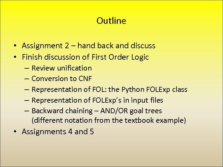 Outline • Assignment 2 – hand back and discuss • Finish discussion of First Order Logic – Review unification – Conversion to CNF – Representation of FOL: the Python FOLExp class – Representation of FOLExp’s in input files – Backward chaining – AND/OR goal trees (different notation from the textbook example) • Assignments 4 and 5
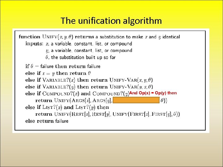 The unification algorithm And Op(x) = Op(y) then
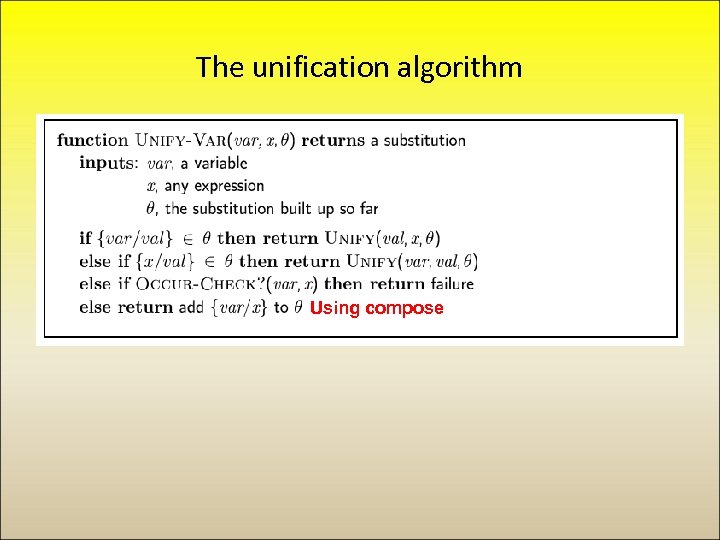 The unification algorithm Using compose
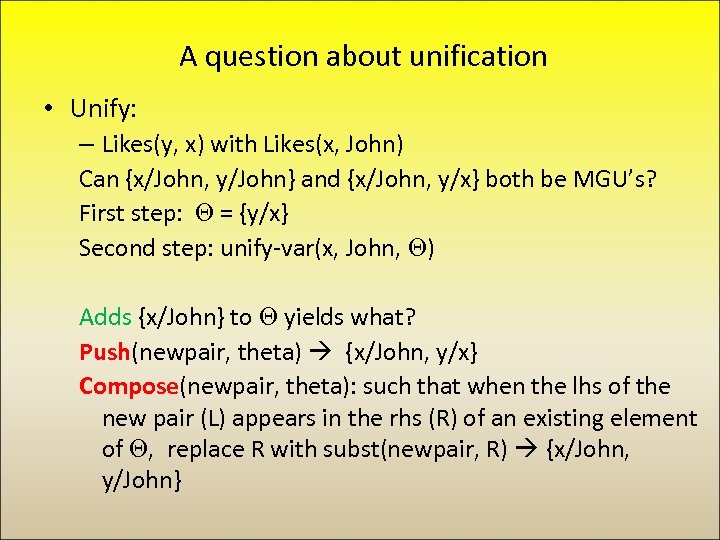 A question about unification • Unify: – Likes(y, x) with Likes(x, John) Can {x/John, y/John} and {x/John, y/x} both be MGU’s? First step: = {y/x} Second step: unify-var(x, John, ) Adds {x/John} to yields what? Push(newpair, theta) {x/John, y/x} Compose(newpair, theta): such that when the lhs of the new pair (L) appears in the rhs (R) of an existing element of , replace R with subst(newpair, R) {x/John, y/John}
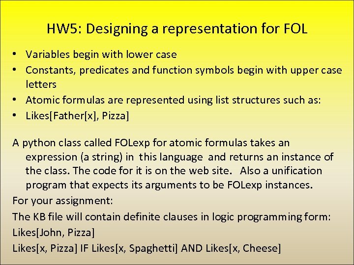 HW 5: Designing a representation for FOL • Variables begin with lower case • Constants, predicates and function symbols begin with upper case letters • Atomic formulas are represented using list structures such as: • Likes[Father[x], Pizza] A python class called FOLexp for atomic formulas takes an expression (a string) in this language and returns an instance of the class. The code for it is on the web site. Also a unification program that expects its arguments to be FOLexp instances. For your assignment: The KB file will contain definite clauses in logic programming form: Likes[John, Pizza] Likes[x, Pizza] IF Likes[x, Spaghetti] AND Likes[x, Cheese]
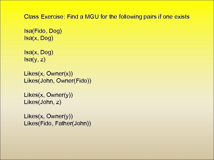 Class Exercise: Find a MGU for the following pairs if one exists Isa(Fido, Dog) Isa(x, Dog) Isa(y, z) Likes(x, Owner(x)) Likes(John, Owner(Fido)) Likes(x, Owner(y)) Likes(John, z) Likes(x, Owner(y)) Likes(Fido, Father(John))
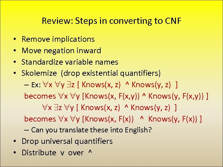 Review: Steps in converting to CNF • • Remove implications Move negation inward Standardize variable names Skolemize (drop existential quantifiers) – Ex: x y z [ Knows(x, z) ^ Knows(y, z) ] becomes x y [Knows(x, F(x, y)) ^ Knows(y, F(x, y)) ] x z y [ Knows(x, z) ^ Knows(y, z) ] becomes x y [Knows(x, F(x)) ^ Knows(y, F(x)) ] – Can you translate these into English? • Drop universal quantifiers • Distribute v over ^
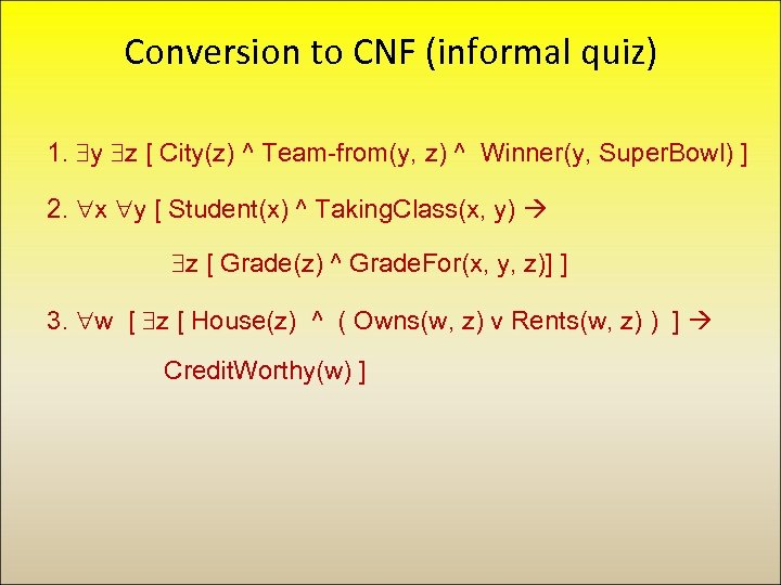 Conversion to CNF (informal quiz) 1. y z [ City(z) ^ Team-from(y, z) ^ Winner(y, Super. Bowl) ] 2. x y [ Student(x) ^ Taking. Class(x, y) z [ Grade(z) ^ Grade. For(x, y, z)] ] 3. w [ z [ House(z) ^ ( Owns(w, z) v Rents(w, z) ) ] Credit. Worthy(w) ]
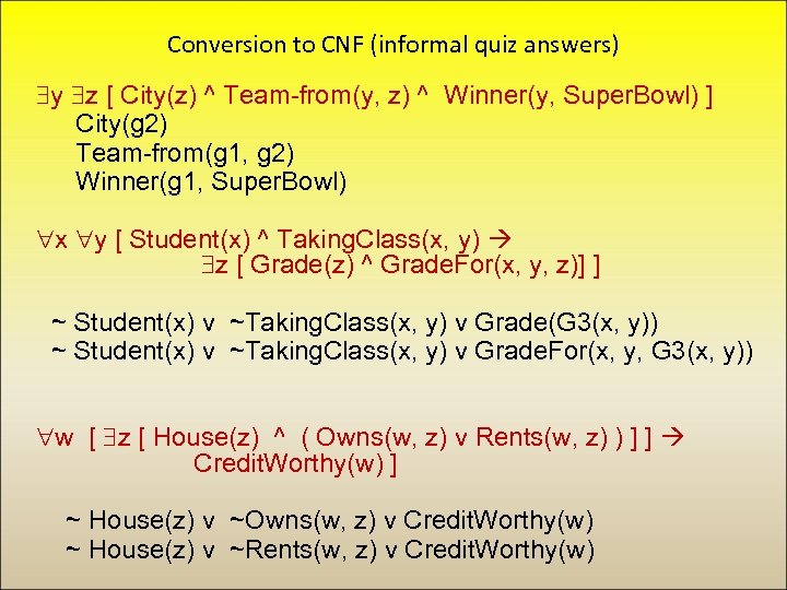 Conversion to CNF (informal quiz answers) y z [ City(z) ^ Team-from(y, z) ^ Winner(y, Super. Bowl) ] City(g 2) Team-from(g 1, g 2) Winner(g 1, Super. Bowl) x y [ Student(x) ^ Taking. Class(x, y) z [ Grade(z) ^ Grade. For(x, y, z)] ] ~ Student(x) v ~Taking. Class(x, y) v Grade(G 3(x, y)) ~ Student(x) v ~Taking. Class(x, y) v Grade. For(x, y, G 3(x, y)) w [ z [ House(z) ^ ( Owns(w, z) v Rents(w, z) ) ] ] Credit. Worthy(w) ] ~ House(z) v ~Owns(w, z) v Credit. Worthy(w) ~ House(z) v ~Rents(w, z) v Credit. Worthy(w)
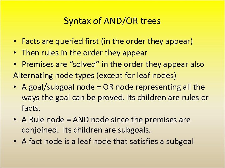 Syntax of AND/OR trees • Facts are queried first (in the order they appear) • Then rules in the order they appear • Premises are “solved” in the order they appear also Alternating node types (except for leaf nodes) • A goal/subgoal node = OR node representing all the ways the goal can be proved. Its children are rules or facts. • A Rule node = AND node since the premises are conjoined. Its children are subgoals. • A fact node is a leaf node that satisfies a subgoal
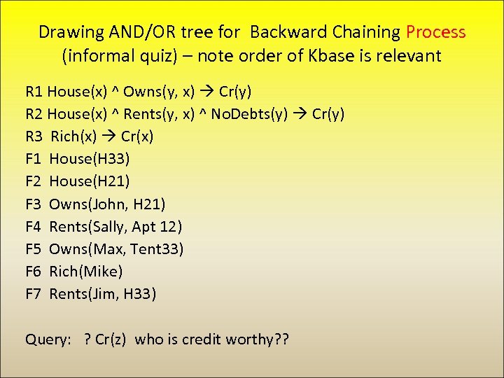 Drawing AND/OR tree for Backward Chaining Process (informal quiz) – note order of Kbase is relevant R 1 House(x) ^ Owns(y, x) Cr(y) R 2 House(x) ^ Rents(y, x) ^ No. Debts(y) Cr(y) R 3 Rich(x) Cr(x) F 1 House(H 33) F 2 House(H 21) F 3 Owns(John, H 21) F 4 Rents(Sally, Apt 12) F 5 Owns(Max, Tent 33) F 6 Rich(Mike) F 7 Rents(Jim, H 33) Query: ? Cr(z) who is credit worthy? ?
![Answers: [ [z=John] , [z=Mike]] CR(z) [z=John, x 1=H 21] R 1 AND House(x Answers: [ [z=John] , [z=Mike]] CR(z) [z=John, x 1=H 21] R 1 AND House(x](https://present5.com/presentation/b734aee4004d6041381ae12bff48717b/image-13.jpg) Answers: [ [z=John] , [z=Mike]] CR(z) [z=John, x 1=H 21] R 1 AND House(x 1) x 1=H 33 R 2 AND FAIL R 3 [z = Mike] AND Owns(z, x 1) OR F 1 OR Rich(z) OR OR House(x 2) F 2 F 3 No. Debts(z) F 6 z = Mike OR OR x 1=H 21 Rents(z, x 2) F 4 F 7 F 5 z=John z=Max x 1=H 21 x 1=Tent 33 = A KB element F 1 x 2=H 33 F 2 x 2=H 21 = A goal
Answers: [ [z=John] , [z=Mike]] CR(z) [z=John, x 1=H 21] R 1 AND House(x 1) x 1=H 33 R 2 AND FAIL R 3 [z = Mike] AND Owns(z, x 1) OR F 1 OR Rich(z) OR OR House(x 2) F 2 F 3 No. Debts(z) F 6 z = Mike OR OR x 1=H 21 Rents(z, x 2) F 4 F 7 F 5 z=John z=Max x 1=H 21 x 1=Tent 33 = A KB element F 1 x 2=H 33 F 2 x 2=H 21 = A goal
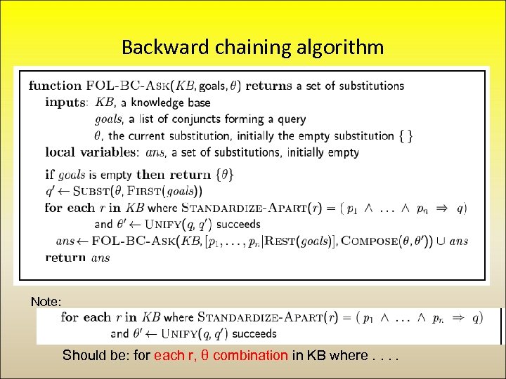 Backward chaining algorithm Note: Should be: for each r, θ combination in KB where. .
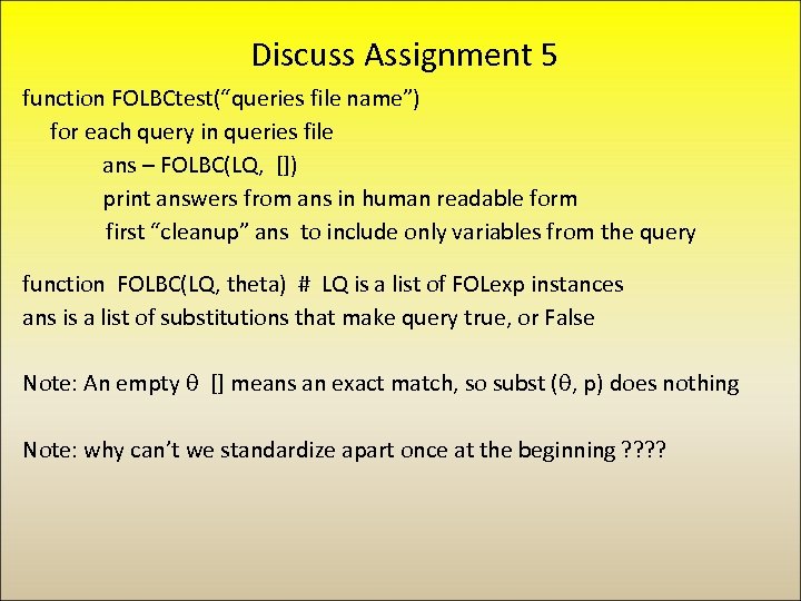 Discuss Assignment 5 function FOLBCtest(“queries file name”) for each query in queries file ans – FOLBC(LQ, []) print answers from ans in human readable form first “cleanup” ans to include only variables from the query function FOLBC(LQ, theta) # LQ is a list of FOLexp instances ans is a list of substitutions that make query true, or False Note: An empty θ [] means an exact match, so subst (θ, p) does nothing Note: why can’t we standardize apart once at the beginning ? ?
 New topic: Search • Classic Search Problems – Missionaries and Cannibals – 8 puzzle – 4 color map problem – Resource allocation/scheduling – Resolution theorem proving – Natural Language parsing – Adversarial games extend the basic model • Relationship to operations research: – Factory scheduling (ex: painting cars) – Logistics (ex: delivering cars to dealers) • Finding optimal or good solutions
 The search framework for problem solving • Given – A set of discrete states (usually finite, but often very large) that define the problem space – A designated start state – One or more states are designated as goal states – A set of operators or actions the agent can perform at each state – A function: Next: State x Op State • Objective: find a sequence of operators that, if applied in the start state, will lead to a goal state • Or: find the shortest or least-cost such sequence
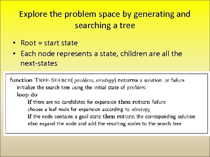 Explore the problem space by generating and searching a tree • Root = start state • Each node represents a state, children are all the next-states
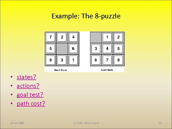 Example: The 8 -puzzle • • states? actions? goal test? path cost? 14 Jan 2004 CS 3243 - Blind Search 19
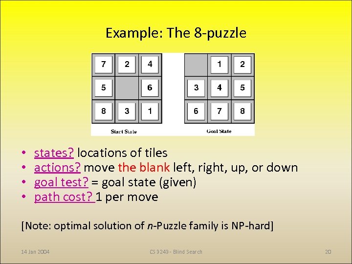 Example: The 8 -puzzle • • states? locations of tiles actions? move the blank left, right, up, or down goal test? = goal state (given) path cost? 1 per move [Note: optimal solution of n-Puzzle family is NP-hard] 14 Jan 2004 CS 3243 - Blind Search 20
 Example: Path Finding • On holiday in Romania; current location is Arad. • Flight leaves tomorrow from Bucharest • A map gives a representation of the problem space • Formulate goal: – Location: Bucharest • Formulate problem: – states: various cities – actions: drive between cities • Find solution: – sequence of cities, e. g. , Arad, Sibiu, Fagaras, Bucharest
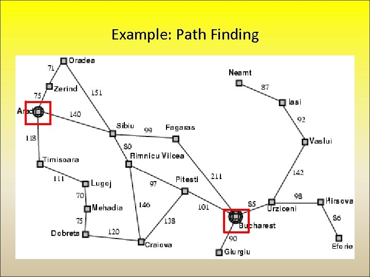 Example: Path Finding
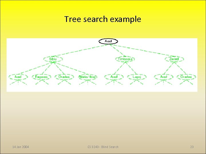 Tree search example 14 Jan 2004 CS 3243 - Blind Search 23
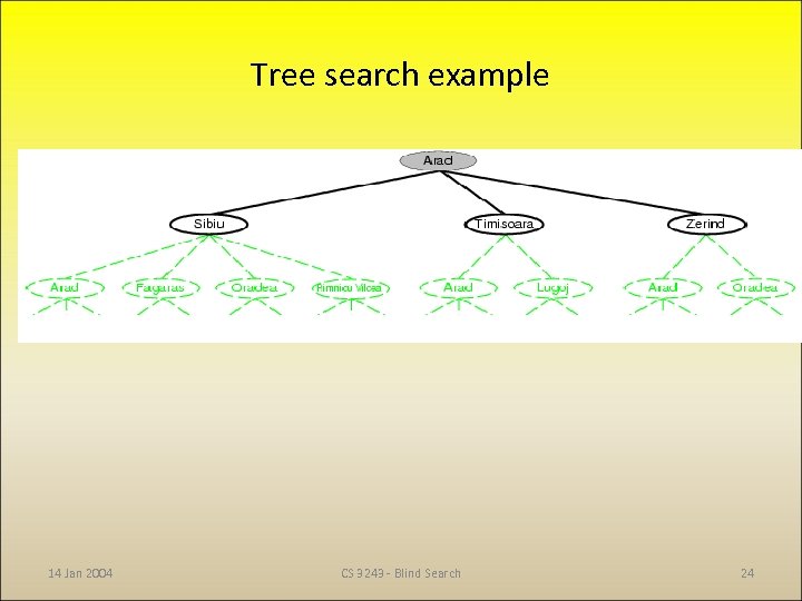 Tree search example 14 Jan 2004 CS 3243 - Blind Search 24
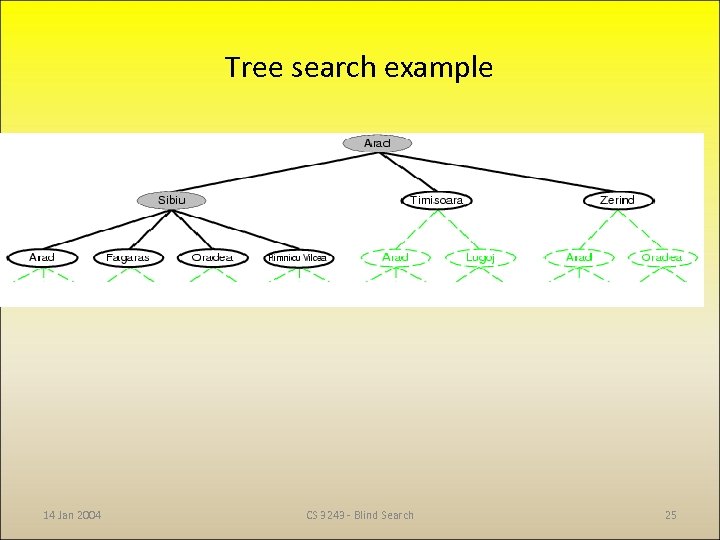 Tree search example 14 Jan 2004 CS 3243 - Blind Search 25
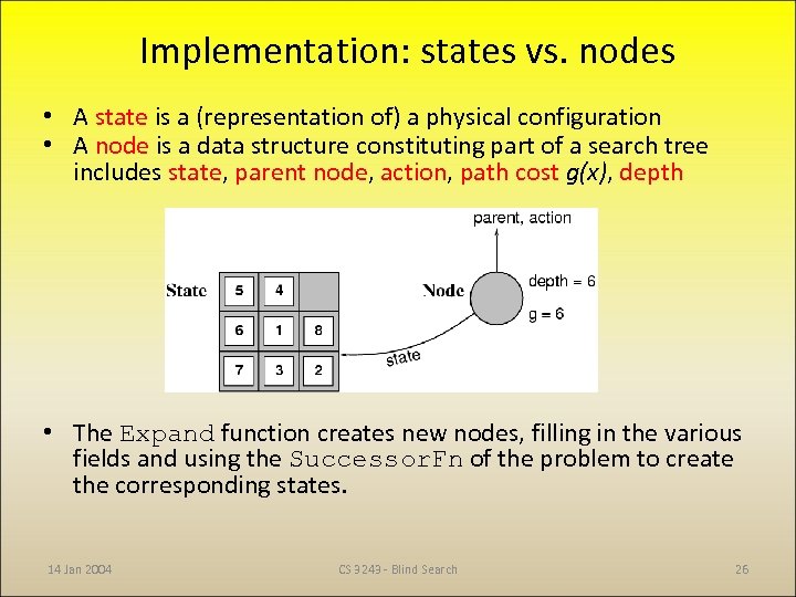 Implementation: states vs. nodes • A state is a (representation of) a physical configuration • A node is a data structure constituting part of a search tree includes state, parent node, action, path cost g(x), depth • The Expand function creates new nodes, filling in the various fields and using the Successor. Fn of the problem to create the corresponding states. 14 Jan 2004 CS 3243 - Blind Search 26
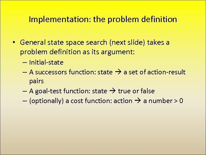 Implementation: the problem definition • General state space search (next slide) takes a problem definition as its argument: – Initial-state – A successors function: state a set of action-result pairs – A goal-test function: state true or false – (optionally) a cost function: action a number > 0
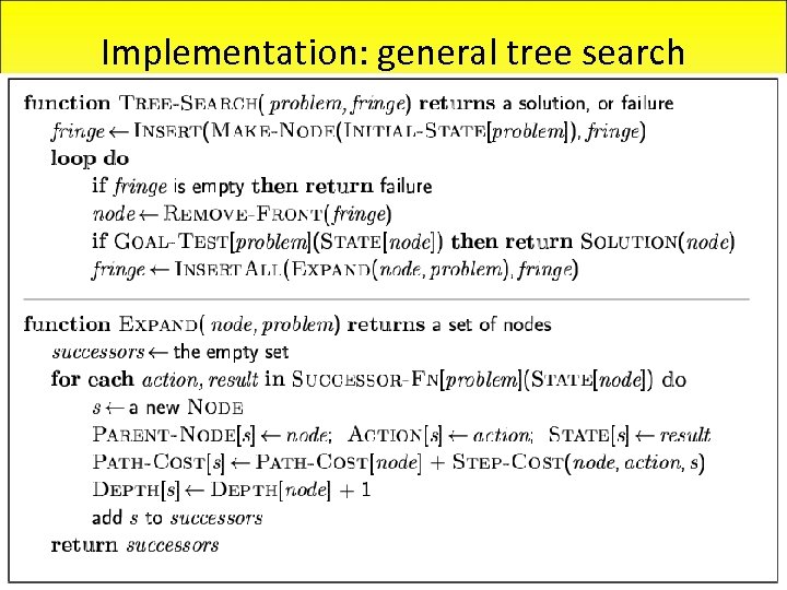 Implementation: general tree search 14 Jan 2004 CS 3243 - Blind Search 28
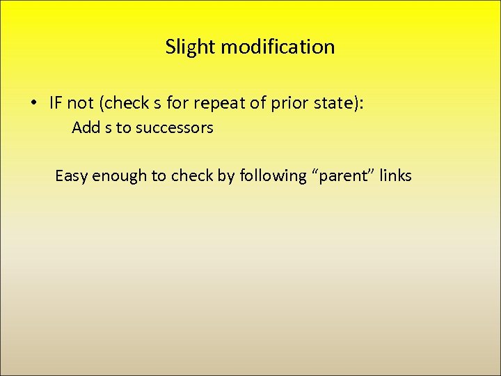 Slight modification • IF not (check s for repeat of prior state): Add s to successors Easy enough to check by following “parent” links
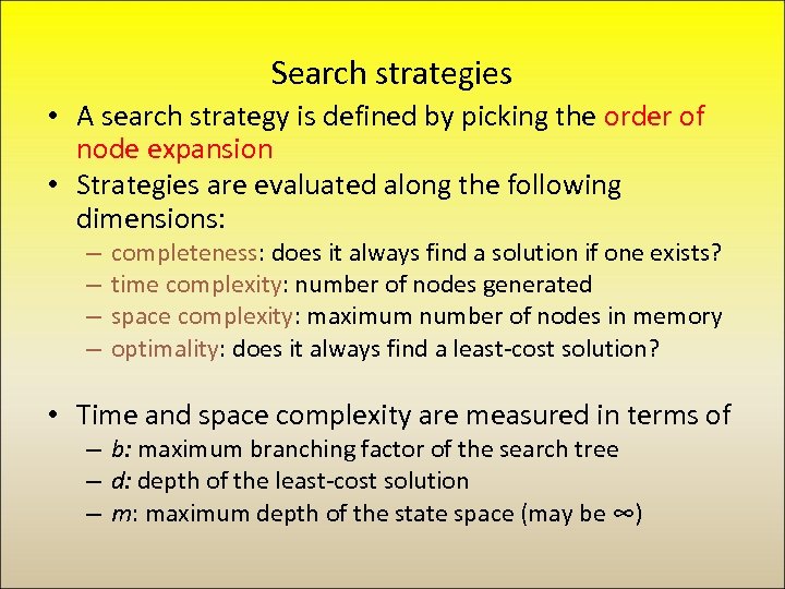 Search strategies • A search strategy is defined by picking the order of node expansion • Strategies are evaluated along the following dimensions: – – completeness: does it always find a solution if one exists? time complexity: number of nodes generated space complexity: maximum number of nodes in memory optimality: does it always find a least-cost solution? • Time and space complexity are measured in terms of – b: maximum branching factor of the search tree – d: depth of the least-cost solution – m: maximum depth of the state space (may be ∞)
 Uninformed search strategies • Uninformed search strategies use only the information available in the problem definition • Breadth-first search • Uniform-cost search • Depth-first search • Depth-limited search • Iterative deepening search
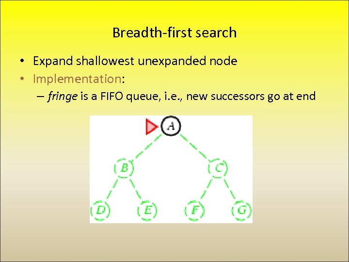 Breadth-first search • Expand shallowest unexpanded node • Implementation: – fringe is a FIFO queue, i. e. , new successors go at end
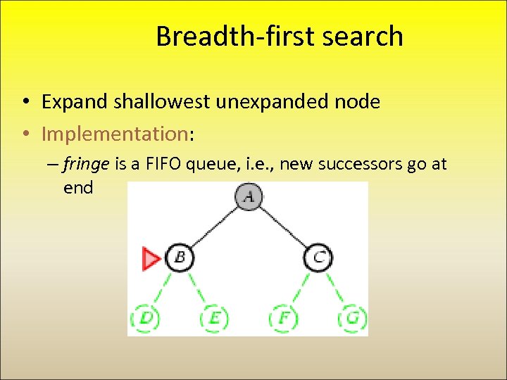 Breadth-first search • Expand shallowest unexpanded node • Implementation: – fringe is a FIFO queue, i. e. , new successors go at end
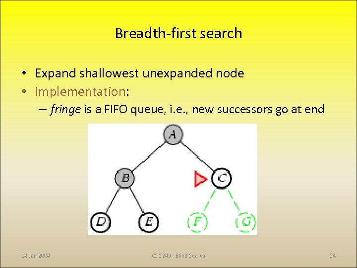 Breadth-first search • Expand shallowest unexpanded node • Implementation: – fringe is a FIFO queue, i. e. , new successors go at end 14 Jan 2004 CS 3243 - Blind Search 34
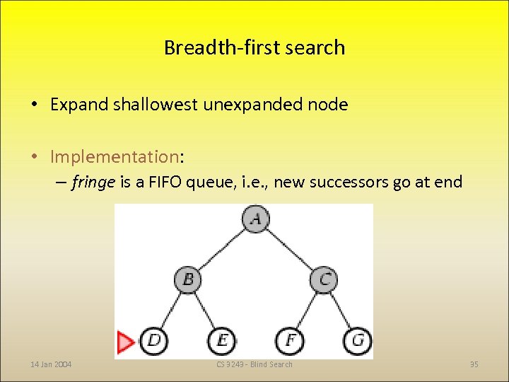 Breadth-first search • Expand shallowest unexpanded node • Implementation: – fringe is a FIFO queue, i. e. , new successors go at end 14 Jan 2004 CS 3243 - Blind Search 35
 Properties of breadth-first search • • Complete? Yes (if b is finite) Time? 1+b+b 2+b 3+… +bd = O(bd+1) Space? O(bd+1) (keeps every node in memory) Optimal? Yes (if cost = 1 per step) • Space is the bigger problem (more than time) Hypothetical in text illustrating the problem of an exponential complexity bound: b (branching factor) = 10, a node uses 1000 bytes, and 10, 000 nodes per second can be generated. A solution at depth 8 takes 31 hours and uses 1 terabyte. At level 9 it is 129 days and 101 terabytes. 14 Jan 2004 CS 3243 - Blind Search 36
 Uniform-cost search • Expand least-cost unexpanded node • Implementation: – fringe = queue ordered by path cost-so-far g(n) • Equivalent to breadth first if step costs are all equal • Complete? Yes, if step cost ≥ ε • Time? # of nodes with g ≤ cost of optimal solution, O(bceiling(C/ ε)) where C is the cost of the optimal solution • Space? The same since all nodes are kept in memory • Optimal? Yes – nodes are expanded in increasing order of g(n)
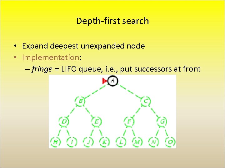 Depth-first search • Expand deepest unexpanded node • Implementation: – fringe = LIFO queue, i. e. , put successors at front
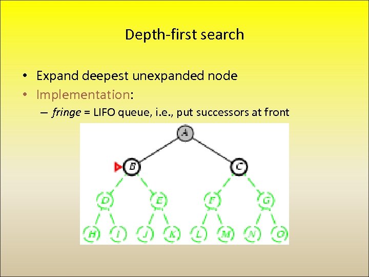 Depth-first search • Expand deepest unexpanded node • Implementation: – fringe = LIFO queue, i. e. , put successors at front
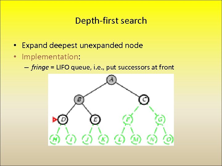 Depth-first search • Expand deepest unexpanded node • Implementation: – fringe = LIFO queue, i. e. , put successors at front
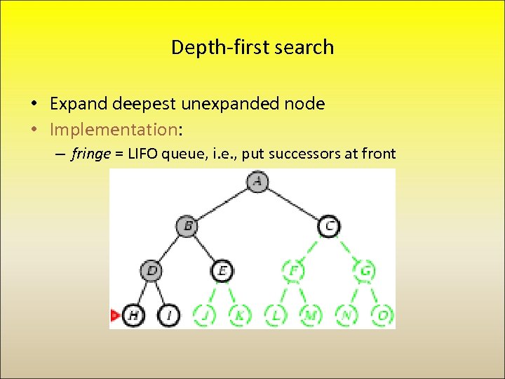 Depth-first search • Expand deepest unexpanded node • Implementation: – fringe = LIFO queue, i. e. , put successors at front
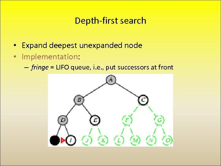 Depth-first search • Expand deepest unexpanded node • Implementation: – fringe = LIFO queue, i. e. , put successors at front
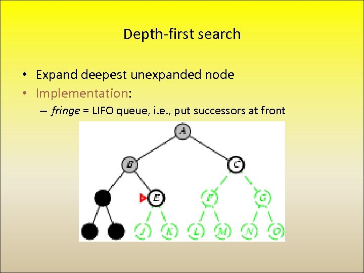 Depth-first search • Expand deepest unexpanded node • Implementation: – fringe = LIFO queue, i. e. , put successors at front
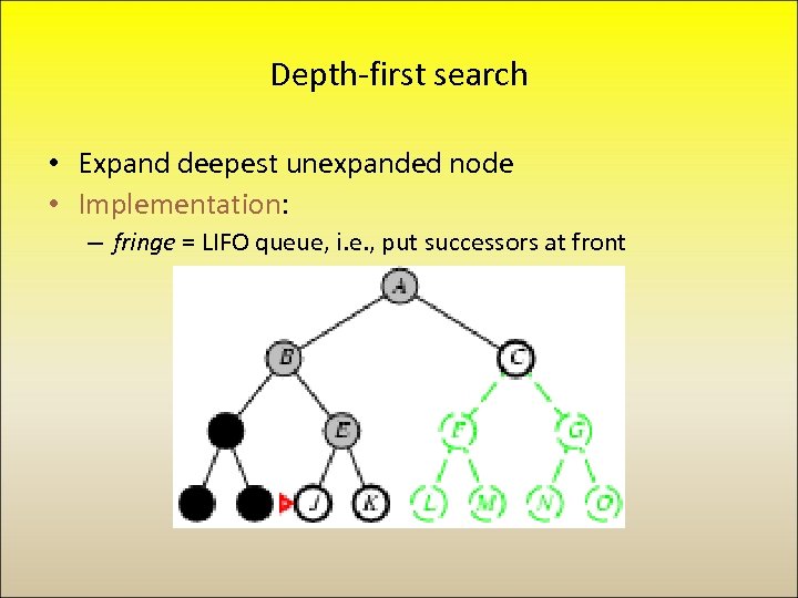 Depth-first search • Expand deepest unexpanded node • Implementation: – fringe = LIFO queue, i. e. , put successors at front
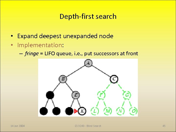 Depth-first search • Expand deepest unexpanded node • Implementation: – fringe = LIFO queue, i. e. , put successors at front 14 Jan 2004 CS 3243 - Blind Search 45
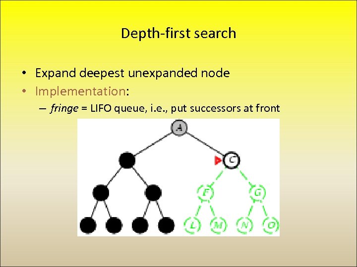 Depth-first search • Expand deepest unexpanded node • Implementation: – fringe = LIFO queue, i. e. , put successors at front
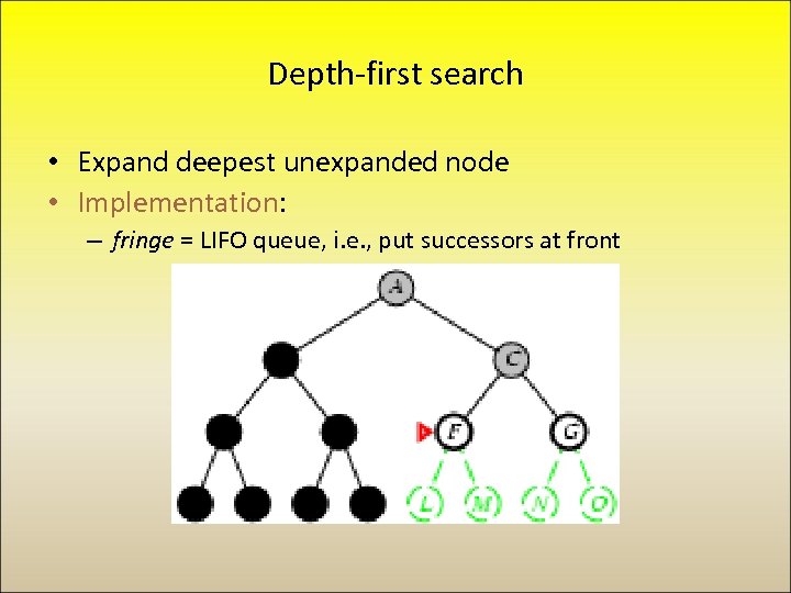 Depth-first search • Expand deepest unexpanded node • Implementation: – fringe = LIFO queue, i. e. , put successors at front
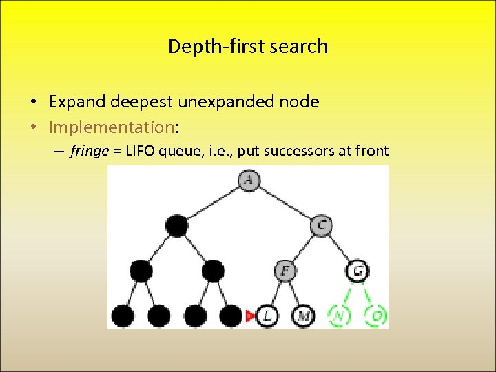 Depth-first search • Expand deepest unexpanded node • Implementation: – fringe = LIFO queue, i. e. , put successors at front
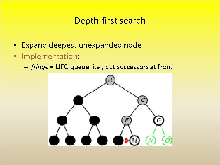 Depth-first search • Expand deepest unexpanded node • Implementation: – fringe = LIFO queue, i. e. , put successors at front
 Properties of depth-first search • Complete? No: fails in infinite-depth spaces • Time? O(bm): terrible if m is much larger than d – but if solutions are dense, may be much faster than breadth-first (m is maximum depth of the state space) • Space? O(bm), i. e. , linear space! • Optimal? No!!
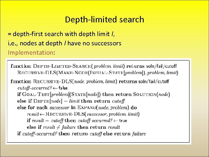 Depth-limited search = depth-first search with depth limit l, i. e. , nodes at depth l have no successors Implementation:
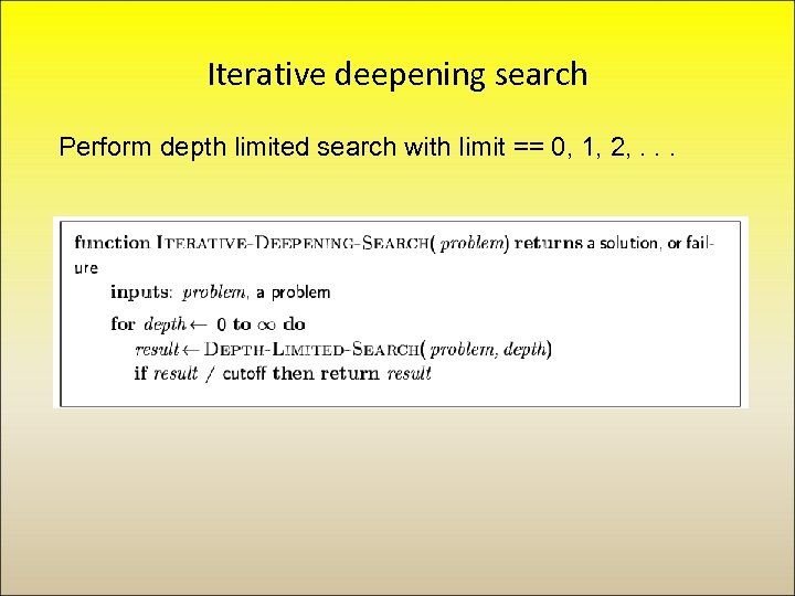 Iterative deepening search Perform depth limited search with limit == 0, 1, 2, . . .
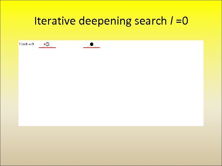 Iterative deepening search l =0
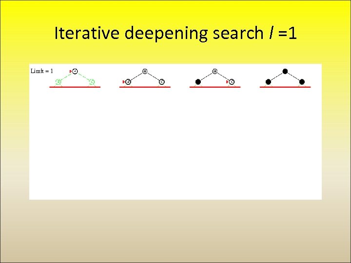 Iterative deepening search l =1
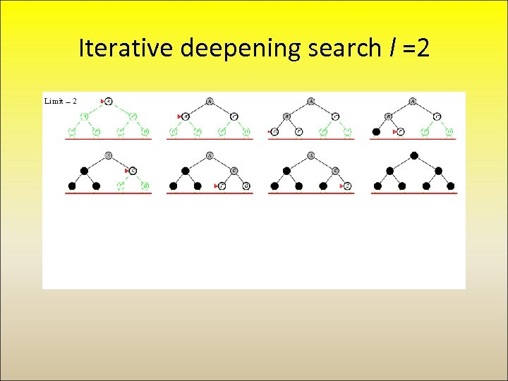 Iterative deepening search l =2
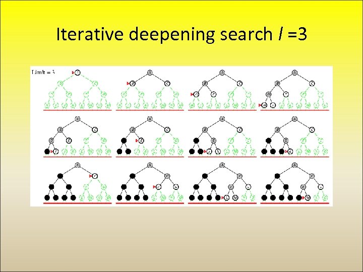 Iterative deepening search l =3
 Iterative deepening search • Number of nodes generated in a depth-limited search to depth d with branching factor b: NDLS = b 0 + b 1 + b 2 + … + bd-2 + bd-1 + bd • Number of nodes generated in an iterative deepening search to depth d with branching factor b: NIDS = (d+1)b 0 + d b 1 + (d-1)b 2 + … + 3 bd-2 +2 bd-1 + 1 bd • For b = 10, d = 5, – NDLS = 1 + 100 + 1, 000 + 100, 000 = 111, 111 – NIDS = 6 + 50 + 400 + 3, 000 + 20, 000 + 100, 000 = 123, 456 • Overhead = (123, 456 - 111, 111)/111, 111 = 11%
 Properties of iterative deepening search • Complete? Yes • Time? (d+1)b 0 + d b 1 + (d-1)b 2 + … + bd = O(bd) – Better than depth first!! • Space? O(bd)– better than depth first! Much better than breadth first • Optimal? Yes, if step cost = 1 • Conclusion: close to the best of both BF and DF
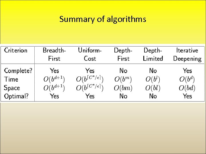 Summary of algorithms
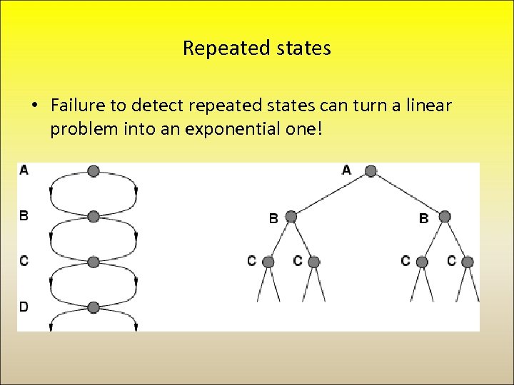 Repeated states • Failure to detect repeated states can turn a linear problem into an exponential one!
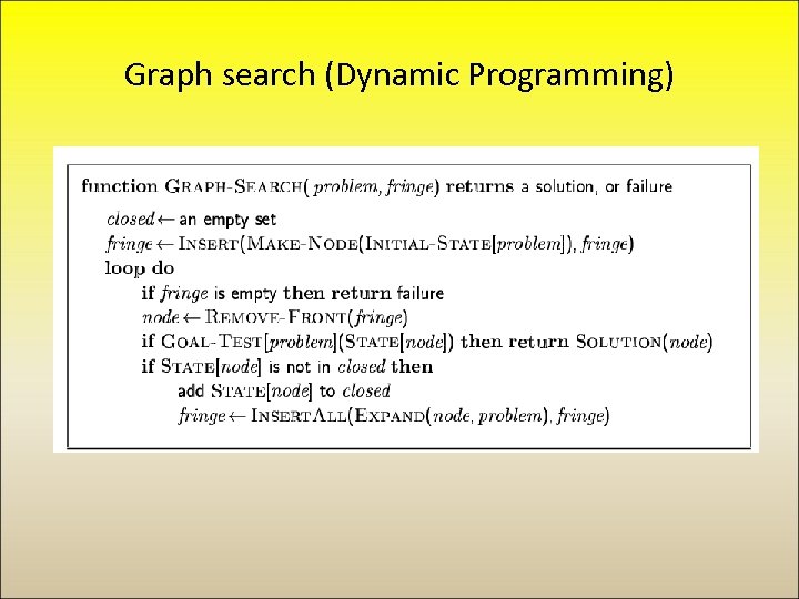 Graph search (Dynamic Programming)
 Informed search algorithms Chapter 3, Section 3. 5
 Outline • • Heuristics Best-first search Greedy best-first search A* search A search strategy is defined by picking the order of node expansion


