3c27b6ff61cba299c8a610bee4e753af.ppt
- Количество слайдов: 59
Credit Analysis, Bond Ratings, Distress Forecast and Financial Information 1
Credit Analysis l The process of evaluating an applicant's loan request or a corporation's debt issue in order to determine the likelihood that the borrower will live up to his/her obligations. 2
Credit Analysis l l Evaluate a borrower’s ability and willingness to repay Questions to address l l l What risks are inherent in the operations of the business? What have managers done or failed to do in mitigating those risks? How can a lender structure and control its own risks in supplying funds? 3
Existing Loan Decisions ØLoan Approvals ØLoan Monitoring ØLoan Terminations 4
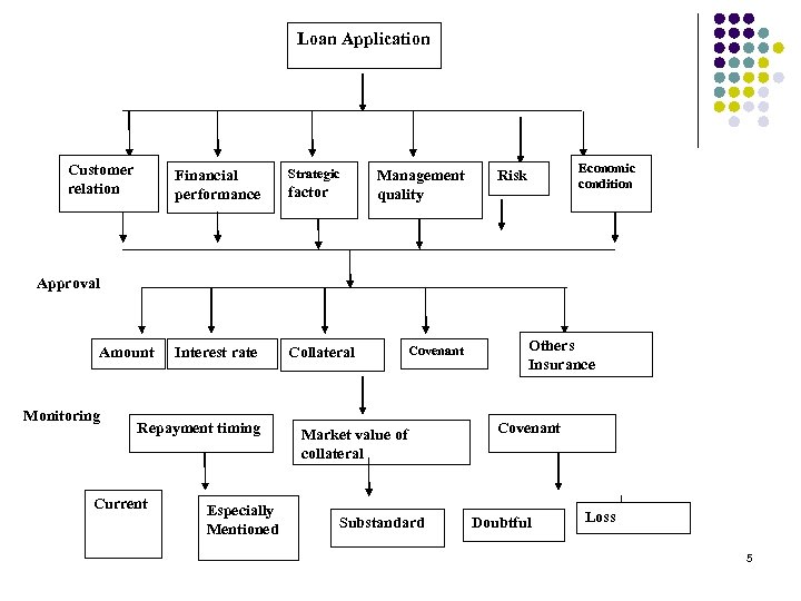
Loan Application Customer relation Financial performance Strategic Interest rate Collateral Yes factor Management quality Economic condition Risk Approval Amount Monitoring Repayment timing Current Especially Mentioned Covenant Market value of collateral Substandard Others Insurance Covenant Doubtful Loss 5
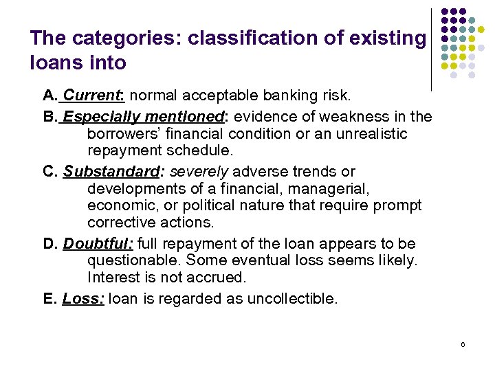
The categories: classification of existing loans into A. Current: normal acceptable banking risk. B. Especially mentioned: evidence of weakness in the borrowers’ financial condition or an unrealistic repayment schedule. C. Substandard: severely adverse trends or developments of a financial, managerial, economic, or political nature that require prompt corrective actions. D. Doubtful: full repayment of the loan appears to be questionable. Some eventual loss seems likely. Interest is not accrued. E. Loss: loan is regarded as uncollectible. 6
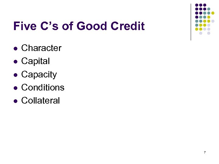
Five C’s of Good Credit l l l Character Capital Capacity Conditions Collateral 7
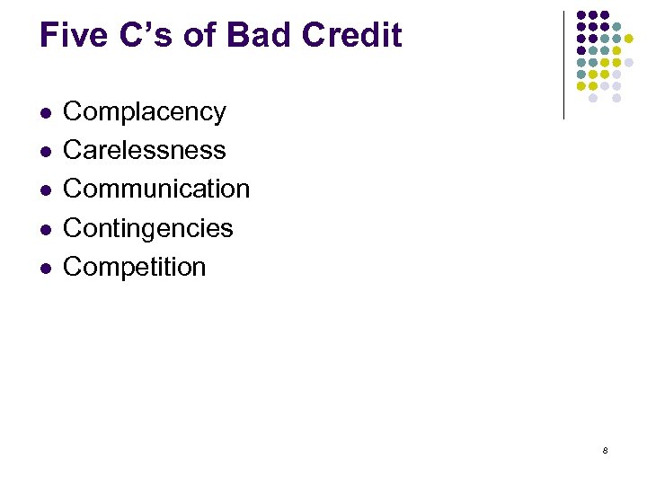
Five C’s of Bad Credit l l l Complacency Carelessness Communication Contingencies Competition 8
Credit Scoring 9
What is credit scoring? l l l A statistical means of providing a quantifiable risk factor for a given customer or applicant. Credit scoring is a process whereby information provided is converted into numbers that are added together to arrive at a score. (“Scorecard”) The objective is to forecast future performance from past behaviour. 10
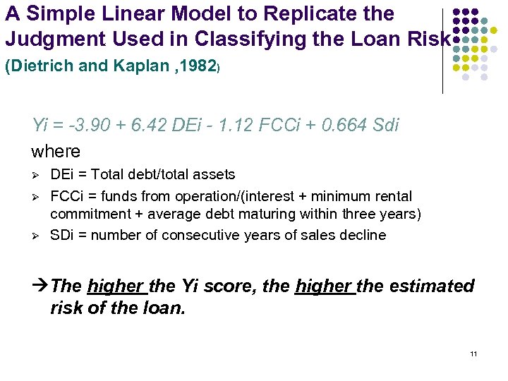
A Simple Linear Model to Replicate the Judgment Used in Classifying the Loan Risk (Dietrich and Kaplan , 1982) Yi = -3. 90 + 6. 42 DEi - 1. 12 FCCi + 0. 664 Sdi where Ø Ø Ø DEi = Total debt/total assets FCCi = funds from operation/(interest + minimum rental commitment + average debt maturing within three years) SDi = number of consecutive years of sales decline The higher the Yi score, the higher the estimated risk of the loan. 11
The hindsight for a simple scoring method l l l The loan officers may consider more than three variables. The loan officers may consider non-linear or nonadditive functional form. The loan officers may consider non financial information. 12
Loss functions for the misclassifications l l Uniform loss function. Loss functions supplied by the bank. 13
The loss function for model prediction errors l l l C 1: (Resulted from type I error) the cost of predicting a loan applicant will not repay when it subsequently repay. It will be contribution margin on the loan that was foregone, assuming that applicants predicted not to repay are refused loans. C 2: (Resulted from type II error) the cost of predicting that a loan applicant will repay when it subsequently does not repay. It will be the loss associated with the interest and principal the bank can not receive when due. Note: Using estimates of C 2 based on loan loss recovery statistics estimated in the 1971 -1975 period, researchers have reported that a C 2 error was 35 times more costly than was a C 1 error. 14
Scoring methods and sample sizes l Ø There is a trade off between having a large enough set of observations to efficiently estimate a scoring method and having a set of firms that are homogeneous with respect to attributes relevant to their loan decision. Solutions: 1. Build a separated scoring system for each industry. But this always resulted in a small sample, especially very few observations for problem loan categories. 2. To control for the hypothesis source of heterogeneity across observations, such as the use of industry relative ratios as a means controlling for differences across industries in their average financial ratios. 15
Credit Analysis and Financial Ratios 16
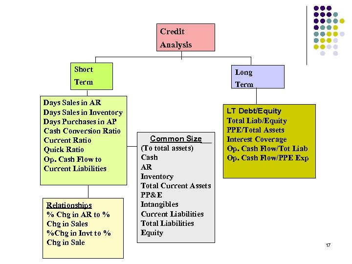
Credit Analysis Short Long Term Days Sales in AR Days Sales in Inventory Days Purchases in AP Cash Conversion Ratio Current Ratio Quick Ratio Op. Cash Flow to Current Liabilities Relationships % Chg in AR to % Chg in Sales %Chg in Invt to % Chg in Sale Common Size (To total assets) Cash AR Inventory Total Current Assets PP&E Intangibles Current Liabilities Total Liabilities Equity LT Debt/Equity Total Liab/Equity PPE/Total Assets Interest Coverage Op. Cash Flow/Tot Liab Op. Cash Flow/PPE Exp 17
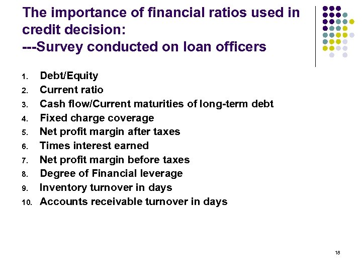
The importance of financial ratios used in credit decision: ---Survey conducted on loan officers 1. 2. 3. 4. 5. 6. 7. 8. 9. 10. Debt/Equity Current ratio Cash flow/Current maturities of long-term debt Fixed charge coverage Net profit margin after taxes Times interest earned Net profit margin before taxes Degree of Financial leverage Inventory turnover in days Accounts receivable turnover in days 18
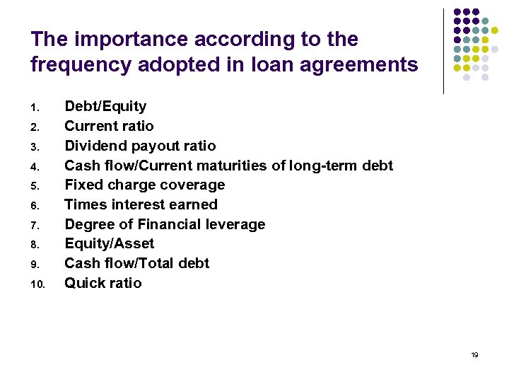
The importance according to the frequency adopted in loan agreements 1. 2. 3. 4. 5. 6. 7. 8. 9. 10. Debt/Equity Current ratio Dividend payout ratio Cash flow/Current maturities of long-term debt Fixed charge coverage Times interest earned Degree of Financial leverage Equity/Asset Cash flow/Total debt Quick ratio 19
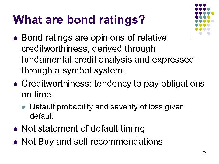
What are bond ratings? l l Bond ratings are opinions of relative creditworthiness, derived through fundamental credit analysis and expressed through a symbol system. Creditworthiness: tendency to pay obligations on time. l l l Default probability and severity of loss given default Not statement of default timing Not Buy and sell recommendations 20
The role of ratings: l Improve the information flow between borrowers and lenders. l l l Minimize monitoring and principal/agent costs l l l Information asymmetry Improve transparency Owners vs managers of firms Fund sponsors vs fund manager Public goods 21
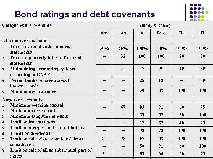
Bond ratings and debt covenants Categories of Covenants Moody’s Rating Aaa Affirmative Covenants 1. Furnish annual audit financial statements 2. Furnish quarterly interim financial statements 3. Maintaining accounting systems according to GAAP 4. Permit banks to have access to books/records 5. Maintaining insurance Negative Covenants 1. Minimum working capital 2. Minimum current ratio 3. Minimum tangible net worth 4. Limit on indebtedness 5. Limit on mergers and consolidations 6. Limits on dividends 7. Limit on sale of stock and/or debt of subsidiaries 8. Limit on sale of all or substantial part of assets Aa A Baa Ba B 50% 66% 100% -- 33 100 80 50 -- -- 17 9 40 50 -- -- 25 18 -- 50 -- -- 50 82 100 -- 67 83 91 60 75 -- -- 33 27 60 100 -- -- 17 27 40 75 -- -- 33 73 100 50 33 67 82 100 -- -- 50 91 60 50 -- 33 64 60 100 22 75
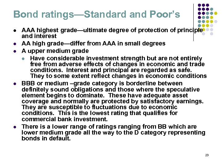
Bond ratings—Standard and Poor’s l l l AAA highest grade—ultimate degree of protection of principle and interest AA high grade—differ from AAA in small degrees A upper medium grade l Have considerable investment strength but are not entirely free from adverse effects of changes in economic and trade conditions. Interest and principal are regarded as safe. They to some extent reflect changes in economic conditions BBB or medium –grade category is borderline between definitely sound obligations and those where the speculative element begins to dominate. These have adequate asset coverage and normally are protected by satisfactory earnings. They are susceptible to fluctuations due to economic conditions. This is the lowest rating that qualifies for commercial bank investment. There is a lower range of ratings ranging from BB which are lower medium grade all the way to the D category representing bonds in default. 23
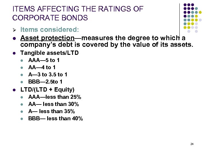
ITEMS AFFECTING THE RATINGS OF CORPORATE BONDS l Items considered: Asset protection—measures the degree to which a company’s debt is covered by the value of its assets. l Tangible assets/LTD Ø l l l AAA— 5 to 1 AA— 4 to 1 A— 3 to 3. 5 to 1 BBB— 2. 5 to 1 LTD/(LTD + Equity) l l AAA—less than 25% AA— less than 30% A— less than 35% BBB— less than 40% 24
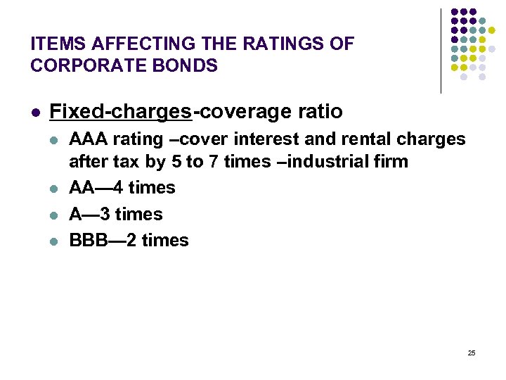
ITEMS AFFECTING THE RATINGS OF CORPORATE BONDS l Fixed-charges-coverage ratio l l AAA rating –cover interest and rental charges after tax by 5 to 7 times –industrial firm AA— 4 times A— 3 times BBB— 2 times 25
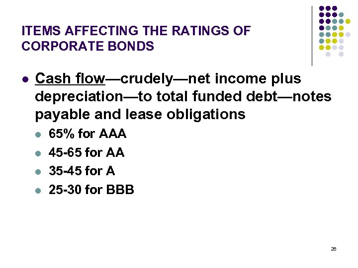
ITEMS AFFECTING THE RATINGS OF CORPORATE BONDS l Cash flow—crudely—net income plus depreciation—to total funded debt—notes payable and lease obligations l l 65% for AAA 45 -65 for AA 35 -45 for A 25 -30 for BBB 26
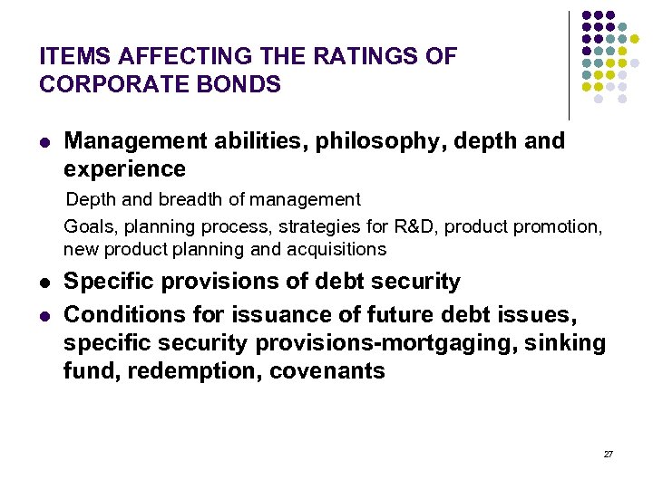
ITEMS AFFECTING THE RATINGS OF CORPORATE BONDS l Management abilities, philosophy, depth and experience Depth and breadth of management Goals, planning process, strategies for R&D, product promotion, new product planning and acquisitions l l Specific provisions of debt security Conditions for issuance of future debt issues, specific security provisions-mortgaging, sinking fund, redemption, covenants 27

Distress Forecast and Financial Information 28
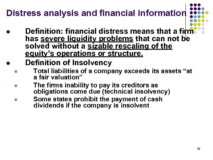
Distress analysis and financial information Definition: financial distress means that a firm has severe liquidity problems that can not be solved without a sizable rescaling of the equity’s operations or structure. Definition of Insolvency l l l Total liabilities of a company exceeds its assets “at a fair valuation” The firms inability to pay its creditors as obligations come due (technical insolvency) Some states prohibit the payment of cash dividends if the company is insolvent 29
Financial Crisis, Some Warning Signals 1. 2. 3. 4. 5. 6. 7. 8. 9. 10. Heavy borrower of working capital Gross margins narrowing Business environment subject to rapid change If volume drops, can production cover expenses Outdated marketing data Organization highly structured/decision time Equipment age/economic downturn Intensity of industry competition Increasing borrowing without an increase in sales Increasing inventory and receivables without an increase in sales 30
Distress analysis and financial information Indicators of financial distress: l l l Cash flow analysis. Corporate strategy analysis. Financial statements of the firm and a set of firms in comparison. External variables such as security returns and bond ratings. 31
Univariate model of distress prediction: involves the use a single variable in prediction model. 32
1. Dichotomous l classification tests: Case study of U. S. Railroad Bankruptcies: Use the ranking of certain variable(s) to predict the bankruptcy of railroad companies. For example, Transportation expenses to operating revenues (TE/OR), and Times interest earned (TIE) 33
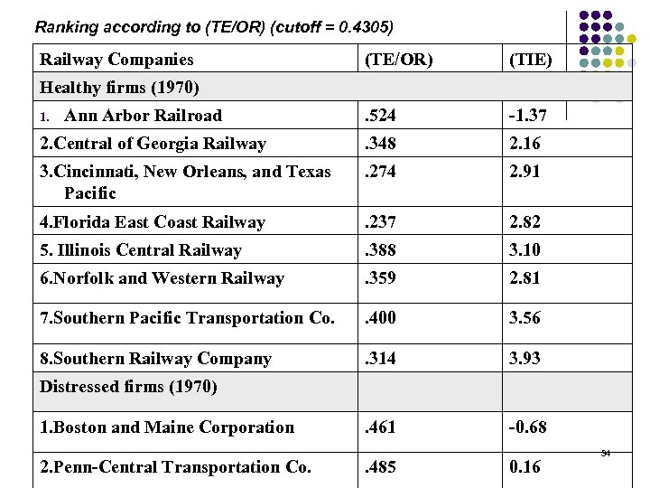
Ranking according to (TE/OR) (cutoff = 0. 4305) Railway Companies (TE/OR) (TIE) . 524 -1. 37 2. Central of Georgia Railway . 348 2. 16 3. Cincinnati, New Orleans, and Texas Pacific . 274 2. 91 4. Florida East Coast Railway . 237 2. 82 5. Illinois Central Railway . 388 3. 10 6. Norfolk and Western Railway . 359 2. 81 7. Southern Pacific Transportation Co. . 400 3. 56 8. Southern Railway Company . 314 3. 93 . 461 -0. 68 Healthy firms (1970) 1. Ann Arbor Railroad Distressed firms (1970) 1. Boston and Maine Corporation 2. Penn-Central Transportation Co. . 485 0. 16 34
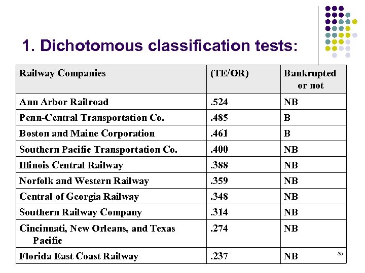
1. Dichotomous classification tests: Railway Companies (TE/OR) Bankrupted or not Ann Arbor Railroad . 524 NB Penn-Central Transportation Co. . 485 B Boston and Maine Corporation . 461 B Southern Pacific Transportation Co. . 400 NB Illinois Central Railway . 388 NB Norfolk and Western Railway . 359 NB Central of Georgia Railway . 348 NB Southern Railway Company . 314 NB Cincinnati, New Orleans, and Texas Pacific . 274 NB Florida East Coast Railway . 237 NB 35
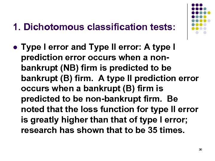
1. Dichotomous classification tests: l Type I error and Type II error: A type I prediction error occurs when a nonbankrupt (NB) firm is predicted to be bankrupt (B) firm. A type II prediction error occurs when a bankrupt (B) firm is predicted to be non-bankrupt firm. Be noted that the loss function for type II error is greatly higher than that of type I error; research has shown that to be 35 times. 36
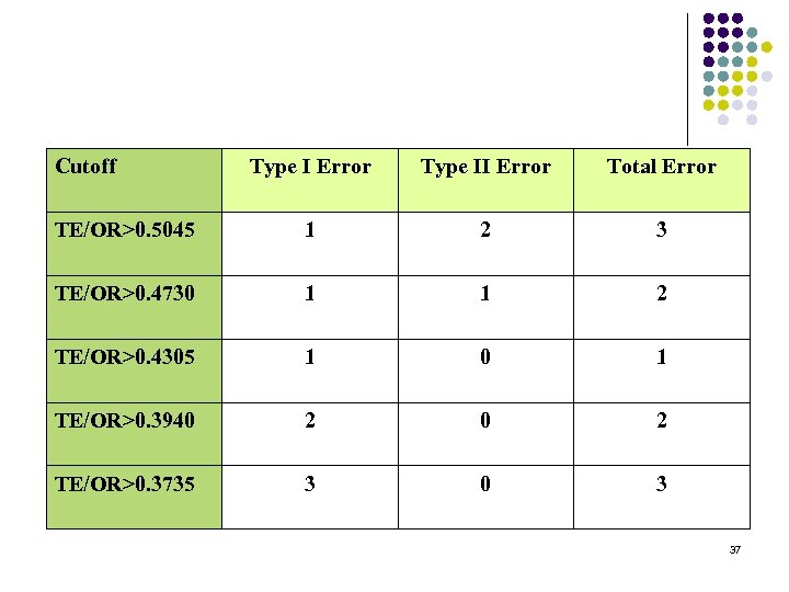
Cutoff Type I Error Type II Error Total Error TE/OR>0. 5045 1 2 3 TE/OR>0. 4730 1 1 2 TE/OR>0. 4305 1 0 1 TE/OR>0. 3940 2 TE/OR>0. 3735 3 0 3 37
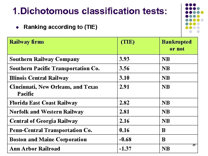
1. Dichotomous classification tests: l Ranking according to (TIE) Railway firms (TIE) Bankrupted or not Southern Railway Company 3. 93 NB Southern Pacific Transportation Co. 3. 56 NB Illinois Central Railway 3. 10 NB Cincinnati, New Orleans, and Texas Pacific 2. 91 NB Florida East Coast Railway 2. 82 NB Norfolk and Western Railway 2. 81 NB Central of Georgia Railway 2. 16 NB Penn-Central Transportation Co. 0. 16 B Boston and Maine Corporation -0. 68 B Ann Arbor Railroad -1. 37 NB 38
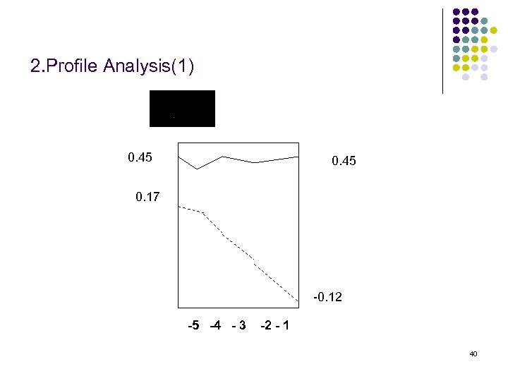
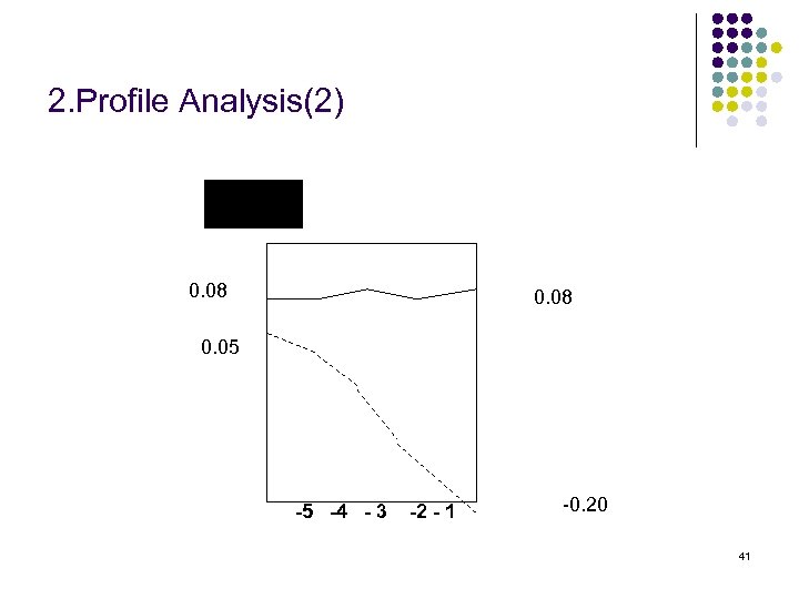
2. Profile Analysis Comparisons of the mean ratios of distress and non-distress firms have been common in bankruptcy prediction. l For each failed firm, a non-fail firm of the same industry and the same asset size was selected. l The equally-weighted means of 30 financial ratios were computed for each of the failed and nonfailed groups in each of the five years before failure. It examines if there are observable differences in the mean ratios of the two sets of firms. l 39
2. Profile Analysis(1) 0. 45 0. 17 -0. 12 -5 -4 - 3 -2 - 1 40
2. Profile Analysis(2) 0. 08 0. 05 -5 -4 - 3 -2 - 1 -0. 20 41
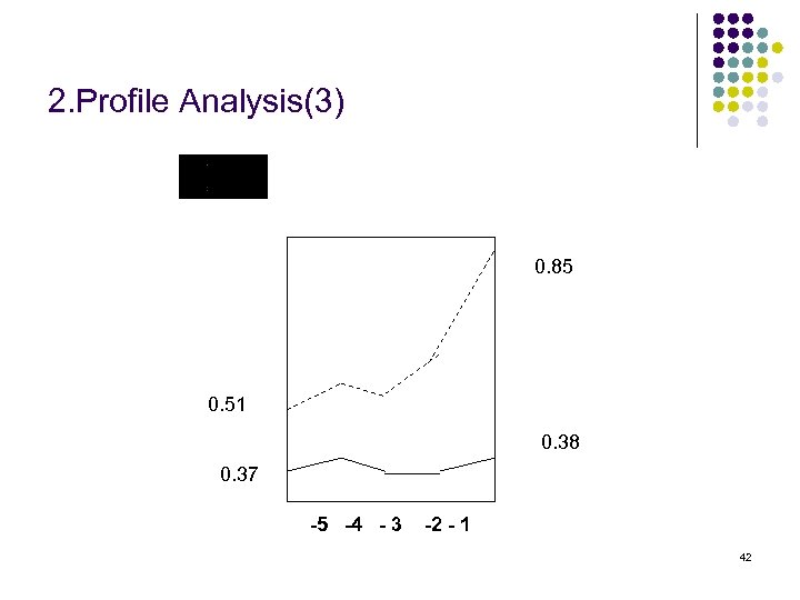
2. Profile Analysis(3) 0. 85 0. 51 0. 38 0. 37 -5 -4 - 3 -2 - 1 42
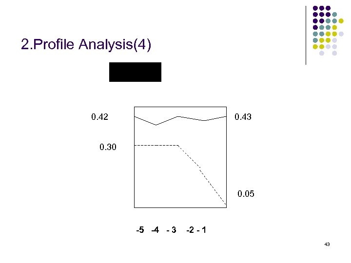
2. Profile Analysis(4) 0. 42 0. 43 0. 30 0. 05 -5 -4 - 3 -2 - 1 43
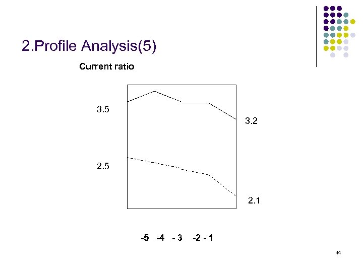
2. Profile Analysis(5) Current ratio 3. 5 3. 2 2. 5 2. 1 -5 -4 - 3 -2 - 1 44
Overview of the uni-variate results There are four categories of variables showing the most consistent difference between bankrupt and non-bankrupt firms were: l l Rate of return Financial leverage Fixed payment coverage Stock return and volatility 45
Multivariate models of distress prediction l l We can use econometric tools by applying more than one financial variables that can effectively discriminate healthy firms from distressed firms. Those tools include Discriminant Analysis, qualitative dependent variable regressions (e. g. Linear probability models, probit regression, and logit regression), and non-linear forecasting tools, such as Neural Network techniques. The dependent variable of these models is either a prediction as to group membership (bankrupt of non-bankrupt), or a probability estimate of group membership (for example, the probability toward bankruptcy). 46
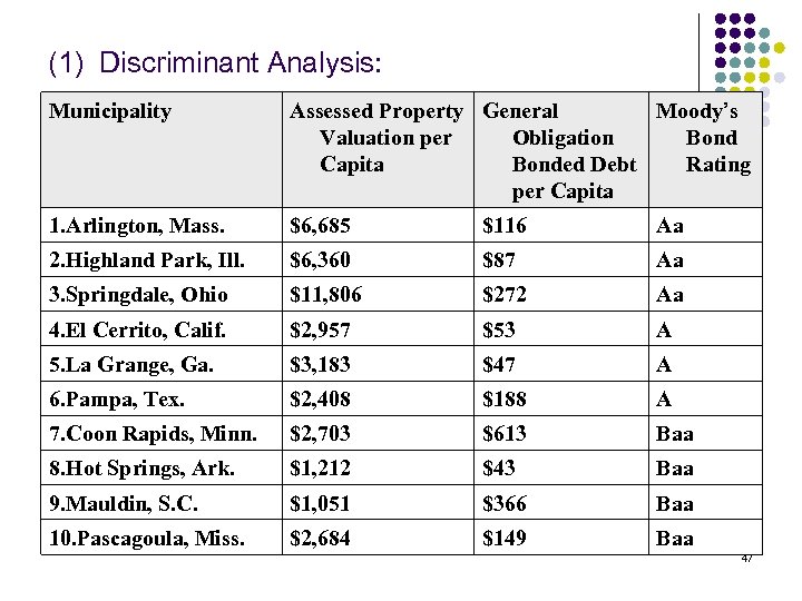
(1) Discriminant Analysis: Municipality Assessed Property General Moody’s Valuation per Obligation Bond Capita Bonded Debt Rating per Capita 1. Arlington, Mass. $6, 685 $116 Aa 2. Highland Park, Ill. $6, 360 $87 Aa 3. Springdale, Ohio $11, 806 $272 Aa 4. El Cerrito, Calif. $2, 957 $53 A 5. La Grange, Ga. $3, 183 $47 A 6. Pampa, Tex. $2, 408 $188 A 7. Coon Rapids, Minn. $2, 703 $613 Baa 8. Hot Springs, Ark. $1, 212 $43 Baa 9. Mauldin, S. C. $1, 051 $366 Baa 10. Pascagoula, Miss. $2, 684 $149 Baa 47
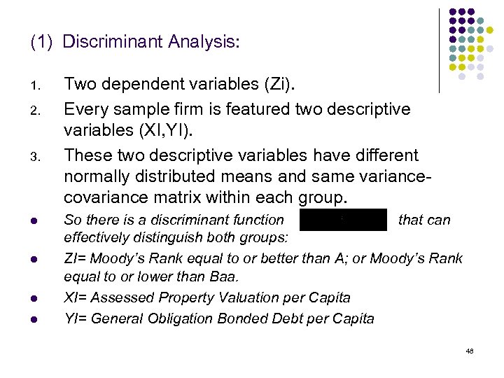
(1) Discriminant Analysis: 1. 2. 3. l l Two dependent variables (Zi). Every sample firm is featured two descriptive variables (XI, YI). These two descriptive variables have different normally distributed means and same variancecovariance matrix within each group. So there is a discriminant function that can effectively distinguish both groups: ZI= Moody’s Rank equal to or better than A; or Moody’s Rank equal to or lower than Baa. XI= Assessed Property Valuation per Capita YI= General Obligation Bonded Debt per Capita 48
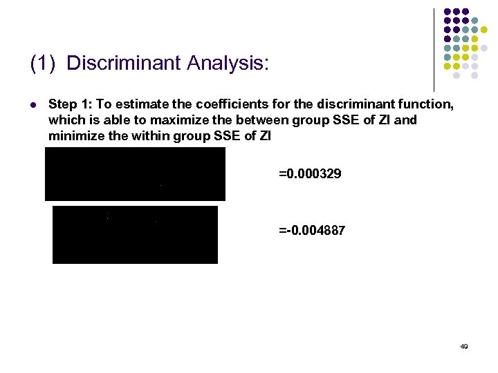
(1) Discriminant Analysis: l Step 1: To estimate the coefficients for the discriminant function, which is able to maximize the between group SSE of ZI and minimize the within group SSE of ZI =0. 000329 =-0. 004887 49
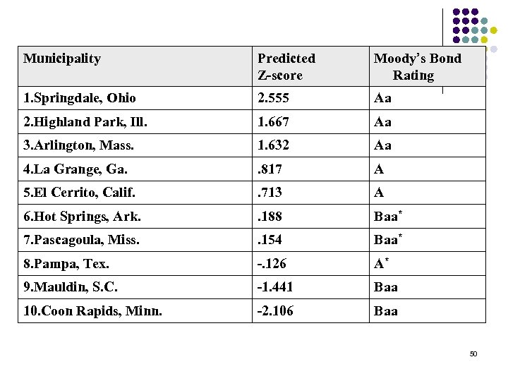
Municipality Predicted Z-score Moody’s Bond Rating 1. Springdale, Ohio 2. 555 Aa 2. Highland Park, Ill. 1. 667 Aa 3. Arlington, Mass. 1. 632 Aa 4. La Grange, Ga. . 817 A 5. El Cerrito, Calif. . 713 A 6. Hot Springs, Ark. . 188 Baa* 7. Pascagoula, Miss. . 154 Baa* 8. Pampa, Tex. -. 126 A* 9. Mauldin, S. C. -1. 441 Baa 10. Coon Rapids, Minn. -2. 106 Baa 50
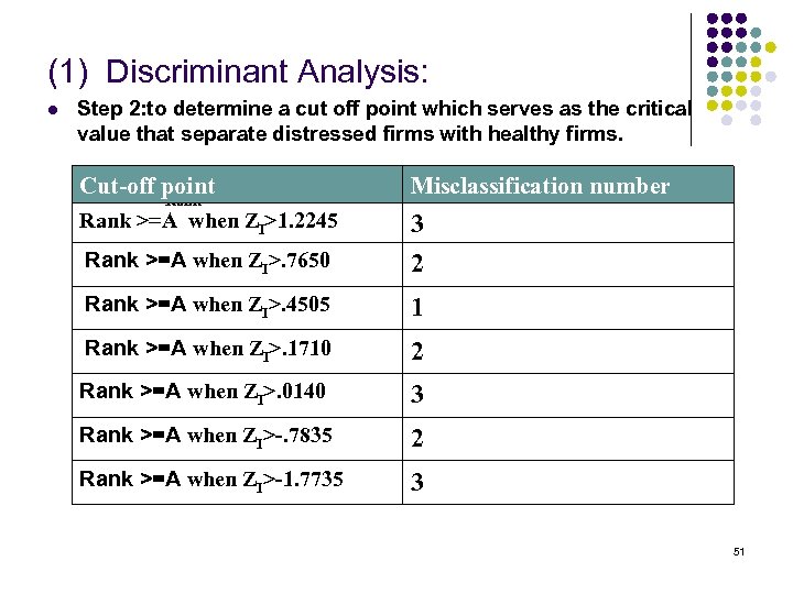
(1) Discriminant Analysis: l Step 2: to determine a cut off point which serves as the critical value that separate distressed firms with healthy firms. Cut-off point Misclassification number Rank >=A when ZI>1. 2245 Rank >=A when ZI>. 7650 3 2 Rank >=A when ZI>. 4505 1 Rank >=A when ZI>. 1710 2 Rank >=A when ZI>. 0140 3 Rank >=A when ZI>-. 7835 2 Rank >=A when ZI>-1. 7735 3 Rank 51
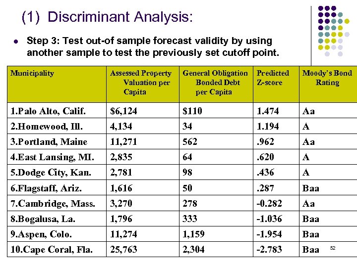
(1) Discriminant Analysis: l Step 3: Test out-of sample forecast validity by using another sample to test the previously set cutoff point. Municipality Assessed Property Valuation per Capita General Obligation Bonded Debt per Capita Predicted Z-score Moody’s Bond Rating 1. Palo Alto, Calif. $6, 124 $110 1. 474 Aa 2. Homewood, Ill. 4, 134 34 1. 194 A 3. Portland, Maine 11, 271 562 . 962 Aa 4. East Lansing, MI. 2, 835 64 . 620 A 5. Dodge City, Kan. 2, 781 98 . 436 A 6. Flagstaff, Ariz. 1, 616 50 . 287 Baa 7. Cambridge, Mass. 3, 270 278 -0. 282 Aa 8. Bogalusa, La. 1, 796 333 -1. 036 Baa 9. Aspen, Colo. 11, 274 1, 159 -1. 954 Baa 10. Cape Coral, Fla. 25, 763 2, 304 -2. 783 Baa 52
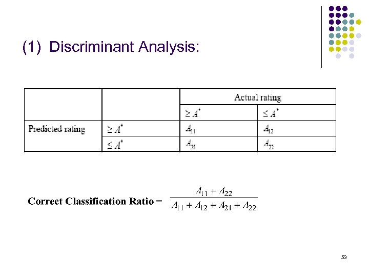
(1) Discriminant Analysis: 53
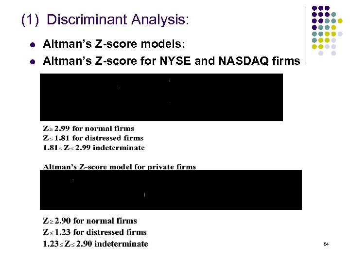
(1) Discriminant Analysis: l l Altman’s Z-score models: Altman’s Z-score for NYSE and NASDAQ firms 54
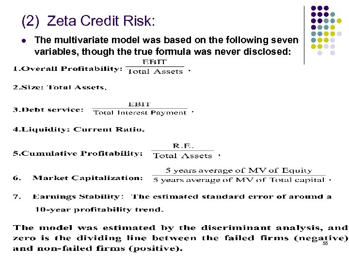
(2) Zeta Credit Risk: l The multivariate model was based on the following seven variables, though the true formula was never disclosed: 55
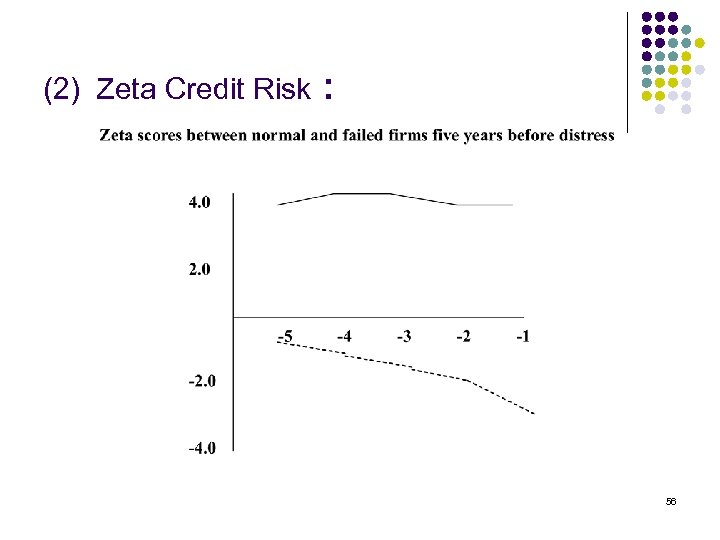
(2) Zeta Credit Risk : 56
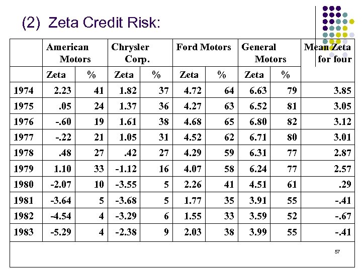
(2) Zeta Credit Risk: American Motors Chrysler Corp. Zeta % Ford Motors Zeta % General Motors Zeta % Mean Zeta for four % 1974 2. 23 41 1. 82 37 4. 72 64 6. 63 79 3. 85 1975 . 05 24 1. 37 36 4. 27 63 6. 52 81 3. 05 1976 -. 60 19 1. 61 38 4. 68 65 6. 80 82 3. 12 1977 -. 22 21 1. 05 31 4. 52 62 6. 71 80 3. 01 1978 . 48 27 . 42 27 4. 29 59 6. 31 77 2. 87 1979 1. 10 33 -1. 12 16 4. 07 58 6. 24 77 2. 57 1980 -2. 07 10 -3. 55 5 2. 26 41 4. 51 61 . 29 1981 -3. 64 5 -3. 68 5 1. 77 35 3. 91 55 -. 41 1982 -4. 54 4 -3. 29 6 1. 55 33 3. 59 52 -. 67 1983 -5. 29 4 -2. 38 9 2. 03 38 3. 99 55 -. 41 57
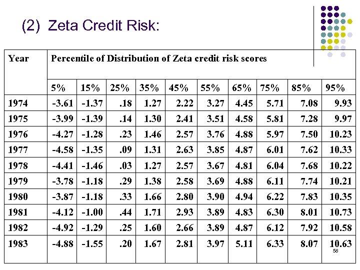
(2) Zeta Credit Risk: Year Percentile of Distribution of Zeta credit risk scores 5% 15% 25% 35% 45% 55% 65% 75% 85% 95% 1974 -3. 61 -1. 37 . 18 1. 27 2. 22 3. 27 4. 45 5. 71 7. 08 9. 93 1975 -3. 99 -1. 39 . 14 1. 30 2. 41 3. 51 4. 58 5. 81 7. 28 9. 97 1976 -4. 27 -1. 28 . 23 1. 46 2. 57 3. 76 4. 88 5. 97 7. 50 10. 23 1977 -4. 58 -1. 35 . 09 1. 31 2. 63 3. 85 4. 87 6. 01 7. 62 10. 33 1978 -4. 41 -1. 46 . 03 1. 27 2. 57 3. 67 4. 81 6. 04 7. 68 10. 22 1979 -3. 78 -1. 18 . 29 1. 38 2. 58 3. 69 4. 88 6. 11 7. 74 10. 21 1980 -3. 87 -1. 18 . 33 1. 66 2. 80 3. 90 4. 94 6. 22 7. 83 10. 35 1981 -4. 12 -1. 00 . 44 1. 71 2. 93 3. 89 4. 83 6. 30 8. 01 10. 73 1982 -4. 92 -1. 29 . 25 1. 60 2. 66 3. 89 4. 87 6. 12 7. 92 10. 58 1983 -4. 88 -1. 55 . 20 1. 67 2. 81 3. 97 5. 11 6. 33 8. 07 10. 63 58
Other devices that predict financial distress l l Qualitative dependent variable regression: probit and logit regressions Artificial Neural Network 59
3c27b6ff61cba299c8a610bee4e753af.ppt