Crash Course in Parallel Computing The why if

Crash Course in Parallel Computing The why, if, when, and how of parallel computing Matt Pedersen (matt@cs. unlv. edu) School of Computer Science

Overview l Why l should we do it? Types of parallel computers l What l should we expect if we do? How fast can we go? l How do we do it? Decomposition l Shared memory vs. message passing l

Overview l Types l of parallel algorithms Data Decomposition Embarrassingly parallel programs l Other examples l l Vibrating string Equation solver Functional Decomposition l Pipeline computation l Should we buy a 5, 000 proc. machine?

Why should we do it? l Need for great computational resources Speed (get things done faster) l Size (solve bigger problems) l l Grand Challenge Problems Global weather forecasting l Modeling large DNA structures l… l

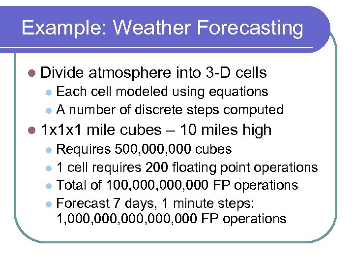Example: Weather Forecasting l Divide atmosphere into 3 -D cells Each cell modeled using equations l A number of discrete steps computed l l 1 x 1 x 1 mile cubes – 10 miles high Requires 500, 000 cubes l 1 cell requires 200 floating point operations l Total of 100, 000, 000 FP operations l Forecast 7 days, 1 minute steps: 1, 000, 000 FP operations l

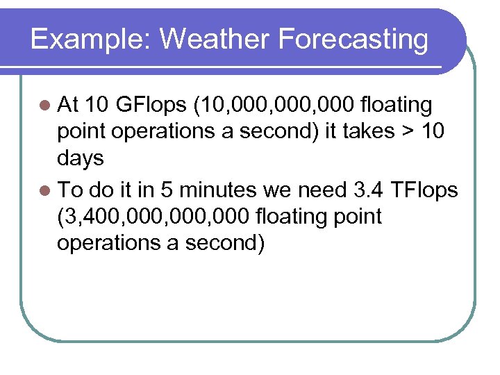Example: Weather Forecasting l At 10 GFlops (10, 000, 000 floating point operations a second) it takes > 10 days l To do it in 5 minutes we need 3. 4 TFlops (3, 400, 000, 000 floating point operations a second)

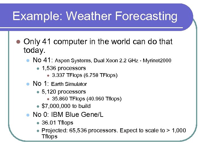Example: Weather Forecasting l Only 41 computer in the world can do that today. l No 41: Aspen Systems, Dual Xeon 2. 2 GHz - Myrinet 2000 l 1, 536 processors l l No 1: Earth Simulator l 5, 120 processors l l l 3. 337 TFlops (6. 758 TFlops) 35. 860 TFlops (40. 960 Tflops) $7, 000 to build No 0: IBM Blue Gene/L l l 36. 01 Tflops Projected: 65, 536 processors. Expect to scale to > 1, 000 Tflops

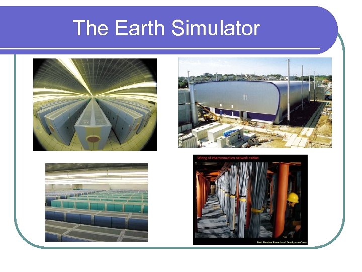The Earth Simulator

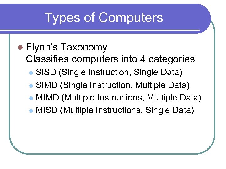Types of Computers l Flynn’s Taxonomy Classifies computers into 4 categories SISD (Single Instruction, Single Data) l SIMD (Single Instruction, Multiple Data) l MIMD (Multiple Instructions, Multiple Data) l MISD (Multiple Instructions, Single Data) l

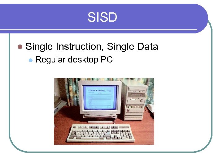SISD l Single l Instruction, Single Data Regular desktop PC

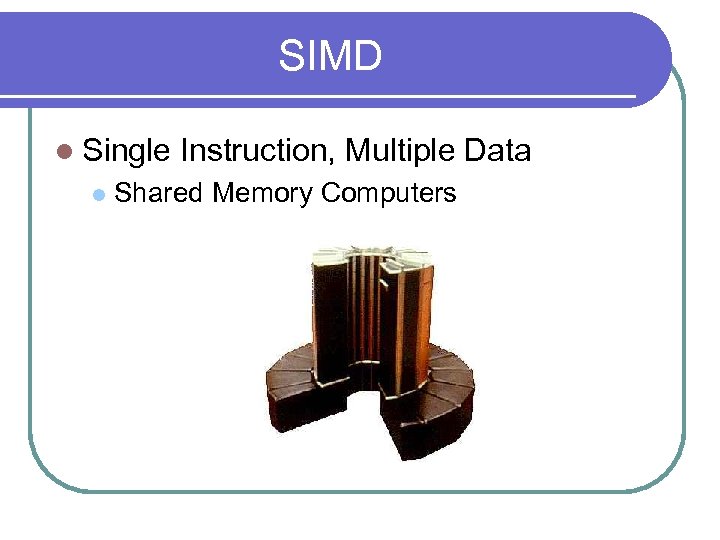SIMD l Single l Instruction, Multiple Data Shared Memory Computers

MISD l Multiple l Instruction, Single Data Does not exist ?

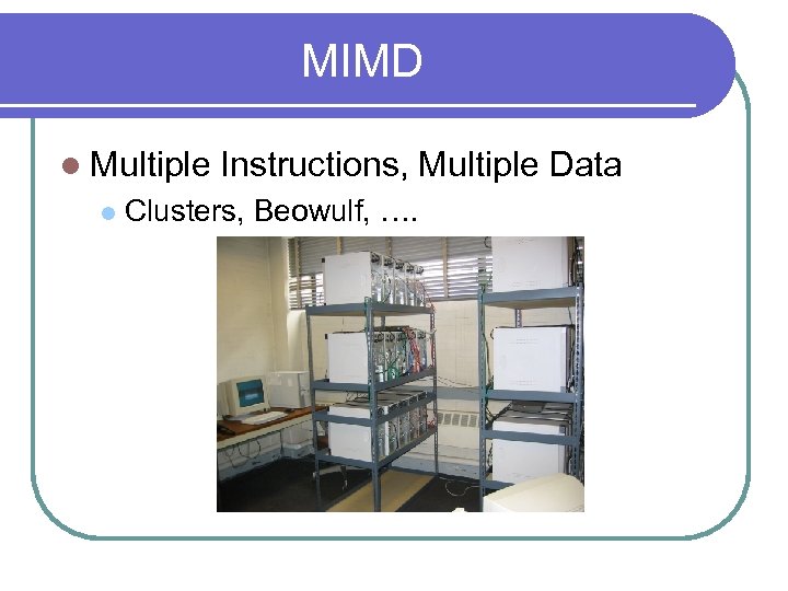MIMD l Multiple l Instructions, Multiple Data Clusters, Beowulf, ….

Clusters (MIMD) l The l future is parallel! (Flynn & Rudd, 96) 19 of 20 fastest computers are clusters Easy to build l ‘Cheap’ l Easy to extend l

What We Want “P processors/computers could provide up to P times the computational power of a single processor, no matter what the current speed of the processor, with the expectation that the problem would be completed in 1/P’th the time”

What We Want vs. What We Get l Parallel l computing is like life: We don’t always get what we want Too many processors might be overkill (Each problem becomes too small) l Some problems do not parallelize well l… l

Speedup l Speedup measures the improvement of using a parallel program over the best sequential program to solve the same problem. Interesting when trying to achieve speed. l Not so interesting if the goal is to solve bigger problems. l

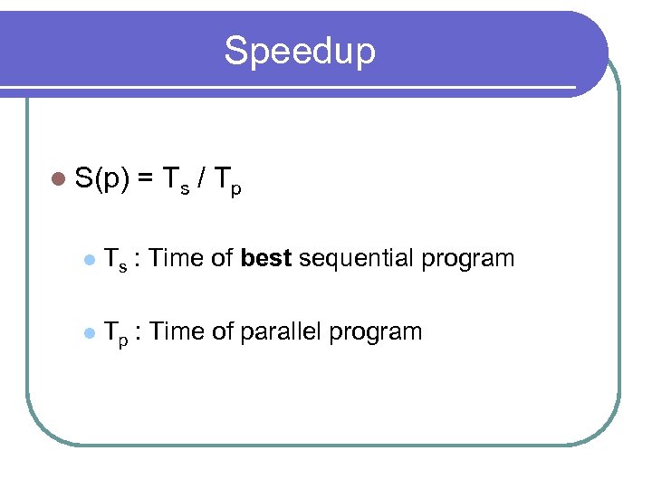Speedup l S(p) = T s / Tp l Ts : Time of best sequential program l Tp : Time of parallel program

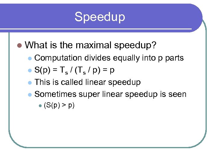Speedup l What is the maximal speedup? Computation divides equally into p parts l S(p) = Ts / (Ts / p) = p l This is called linear speedup l Sometimes super linear speedup is seen l l (S(p) > p)

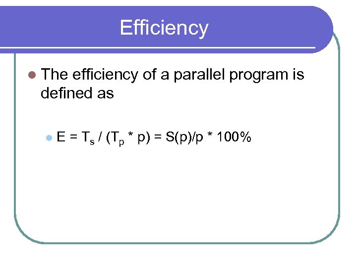Efficiency l The efficiency of a parallel program is defined as l E = Ts / (Tp * p) = S(p)/p * 100%

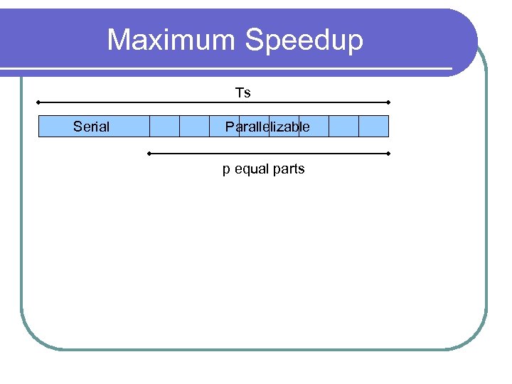
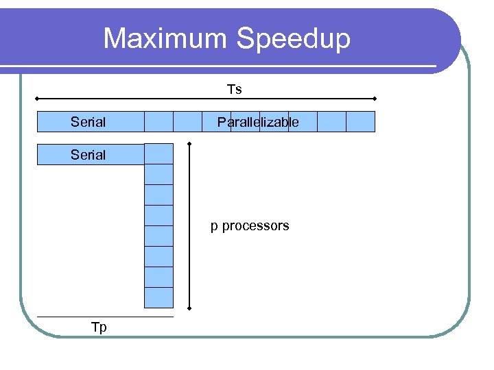
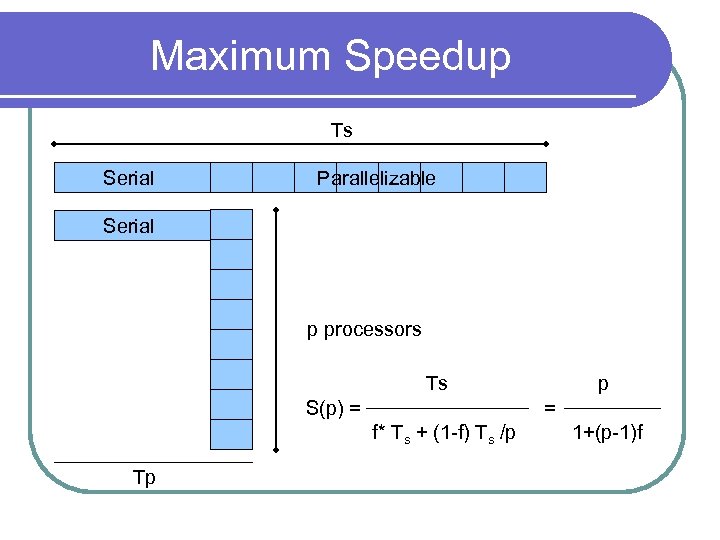
Maximum Speedup l Several things can reduce speedup Idle processors l Extra computation (not in sequential algorithm) l Communication between processes l l. A fraction (f) of most programs cannot be done in parallel

Maximum Speedup Ts Serial Parallelizable

Maximum Speedup Ts Serial Parallelizable p equal parts

Maximum Speedup Ts Serial Parallelizable Serial p processors Tp

Maximum Speedup Ts Serial Parallelizable Serial p processors Ts S(p) = = f* Ts + (1 -f) Ts /p Tp p 1+(p-1)f

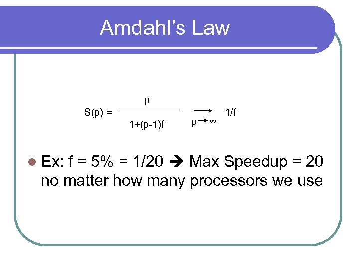Amdahl’s Law p S(p) = 1+(p-1)f l Ex: p ∞ 1/f f = 5% = 1/20 Max Speedup = 20 no matter how many processors we use

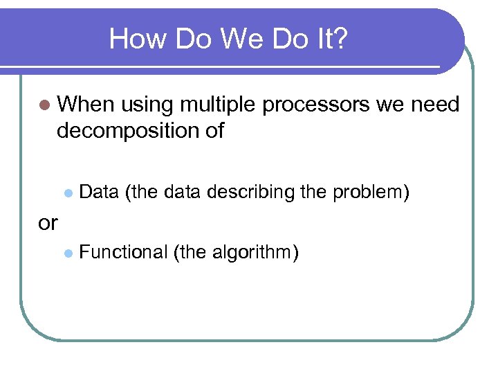How Do We Do It? l When using multiple processors we need decomposition of l Data (the data describing the problem) l Functional (the algorithm) or

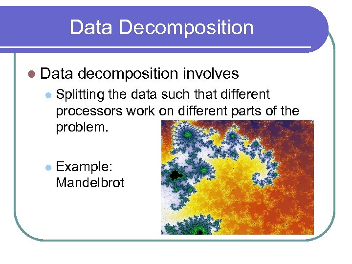Data Decomposition l Data decomposition involves l Splitting the data such that different processors work on different parts of the problem. l Example: Mandelbrot

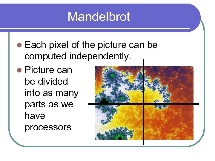Mandelbrot l Each pixel of the picture can be computed independently. l Picture can be divided into as many parts as we have processors

Mandelbrot l No dependencies between pixels l Processes can work independent of each other l In theory, this should parallelize well

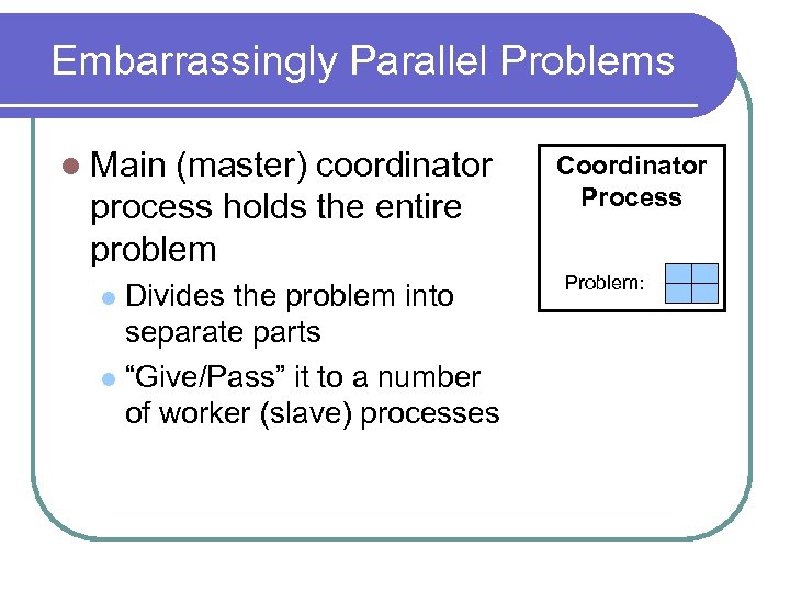Embarrassingly Parallel Problems l Main (master) coordinator process holds the entire problem Divides the problem into separate parts l “Give/Pass” it to a number of worker (slave) processes l Coordinator Process Problem:

Passing Data l Shared memory between all processors Each processor simply uses one part of the memory. l BUT, clusters do not (normally) have shared memory l l Distributed memory Each processor has its own memory l Data must be ‘sent’ and ‘received’ l This is called message passing l

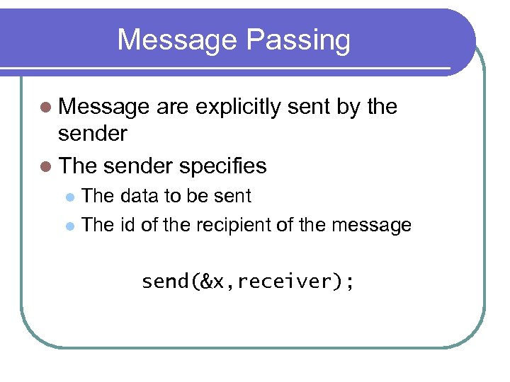Message Passing l Message are explicitly sent by the sender l The sender specifies The data to be sent l The id of the recipient of the message l send(&x, receiver);

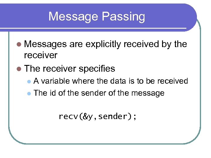Message Passing l Messages are explicitly received by the receiver l The receiver specifies A variable where the data is to be received l The id of the sender of the message l recv(&y, sender);

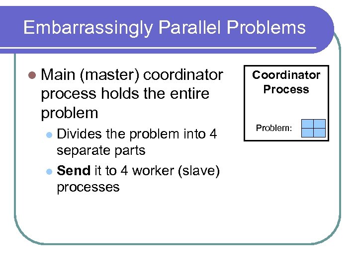Embarrassingly Parallel Problems l Main (master) coordinator process holds the entire problem Divides the problem into 4 separate parts l Send it to 4 worker (slave) processes l Coordinator Process Problem:

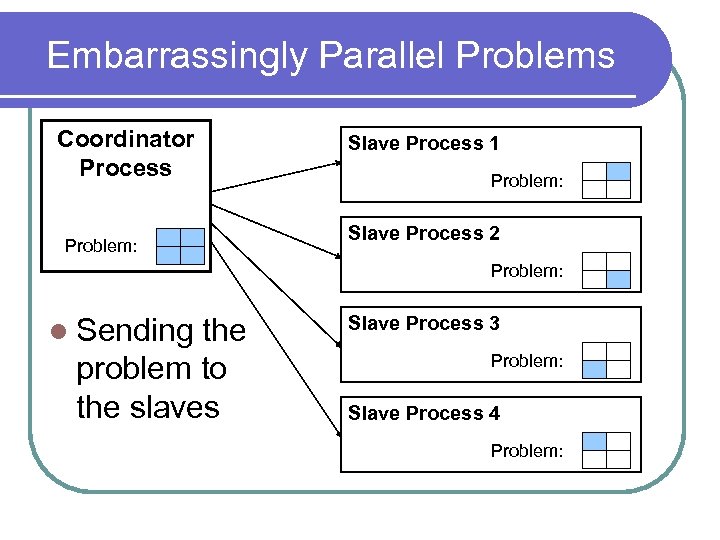Embarrassingly Parallel Problems Coordinator Process Problem: Slave Process 1 Problem: Slave Process 2 Problem: l Sending the problem to the slaves Slave Process 3 Problem: Slave Process 4 Problem:

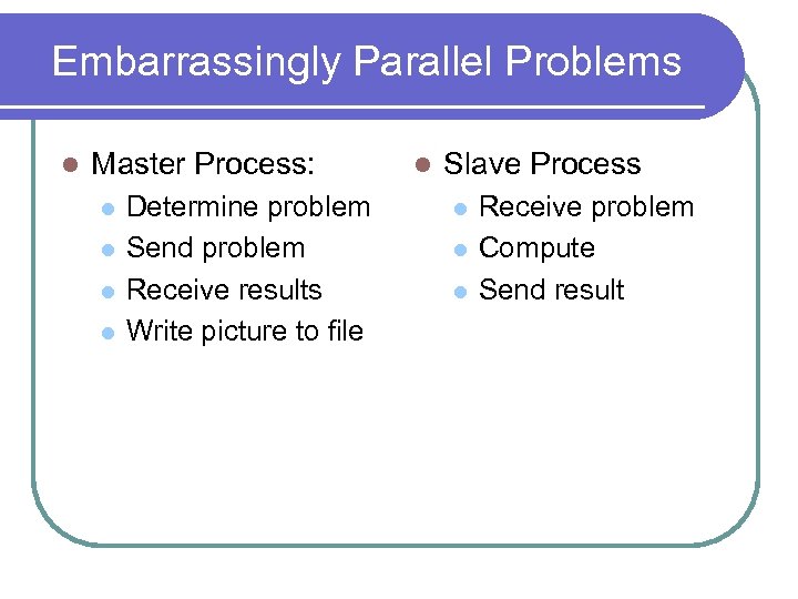Embarrassingly Parallel Problems l Master Process: l l Determine problem Send problem Receive results Write picture to file l Slave Process l l l Receive problem Compute Send result

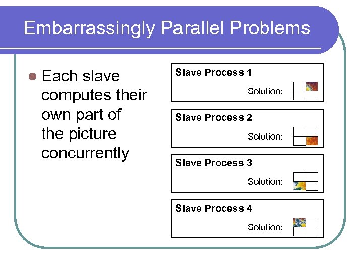Embarrassingly Parallel Problems l Each slave computes their own part of the picture concurrently Slave Process 1 Solution: Slave Process 2 Solution: Slave Process 3 Solution: Slave Process 4 Solution:

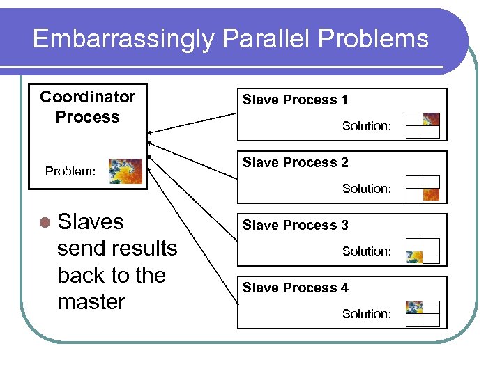Embarrassingly Parallel Problems Coordinator Process Problem: Slave Process 1 Solution: Slave Process 2 Solution: l Slaves send results back to the master Slave Process 3 Solution: Slave Process 4 Solution:

Embarrassingly Parallel Problems l Speedup of embarrassingly parallel problems l The computation part of the program scales linearly If all slaves are equally fast l If all slaves get data representing a problem of equal size l l Not the case with Mandelbrot (black spots take longer to compute than not black)

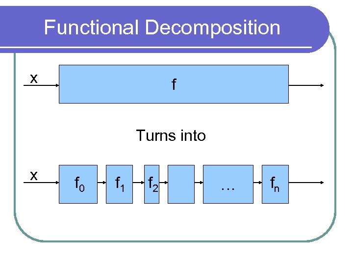
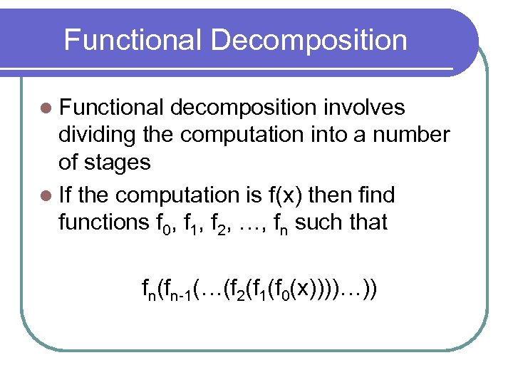Functional Decomposition l Functional decomposition involves dividing the computation into a number of stages l If the computation is f(x) then find functions f 0, f 1, f 2, …, fn such that fn(fn-1(…(f 2(f 1(f 0(x))))…))

Functional Decomposition x f Turns into x f 0 f 1 f 2 … fn

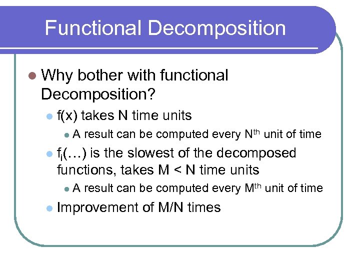Functional Decomposition l Why bother with functional Decomposition? l f(x) takes N time units l A result can be computed every Nth unit of time l fi(…) is the slowest of the decomposed functions, takes M < N time units l l A result can be computed every Mth unit of time Improvement of M/N times

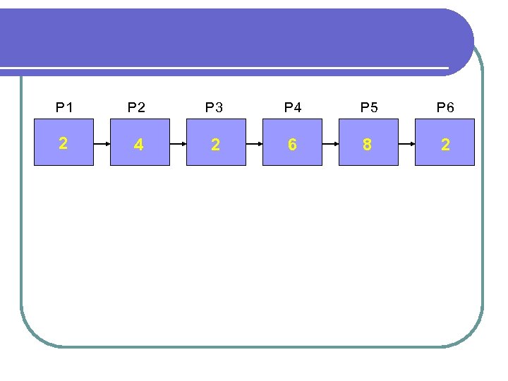
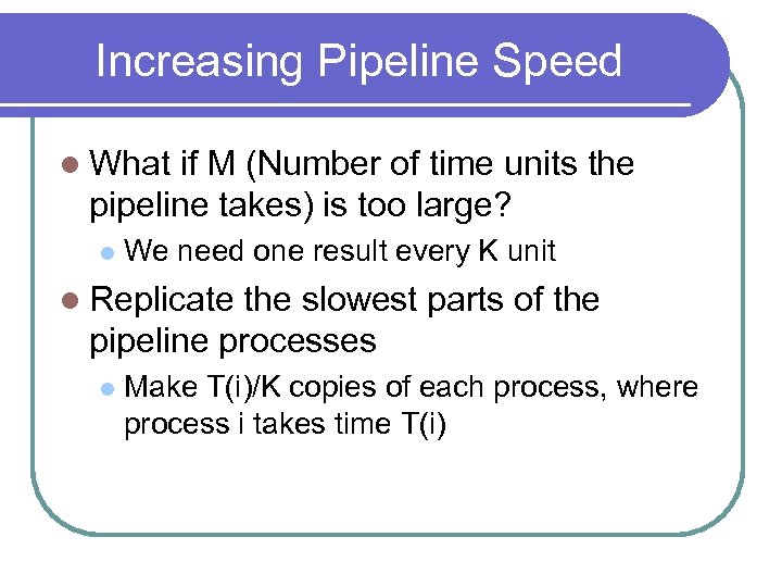Increasing Pipeline Speed l What if M (Number of time units the pipeline takes) is too large? l We need one result every K unit l Replicate the slowest parts of the pipeline processes l Make T(i)/K copies of each process, where process i takes time T(i)

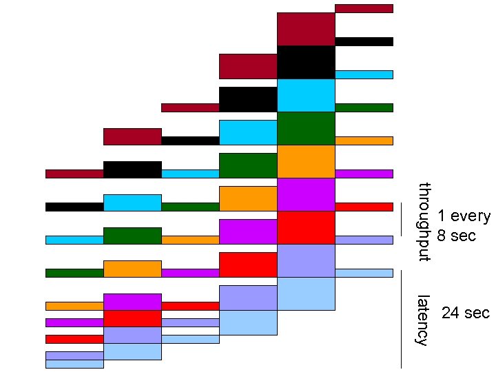
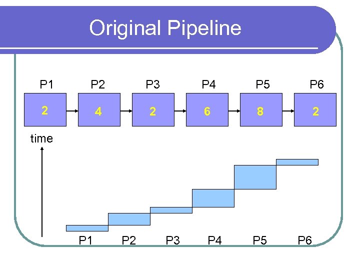Original Pipeline P 1 P 2 P 3 P 4 P 5 P 6 2 4 2 6 8 2 time P 1 P 2 P 3 P 4 P 5 P 6

throughput 1 every 8 sec latency 24 sec

P 1 P 2 P 3 P 4 P 5 P 6 2 4 2 6 8 2

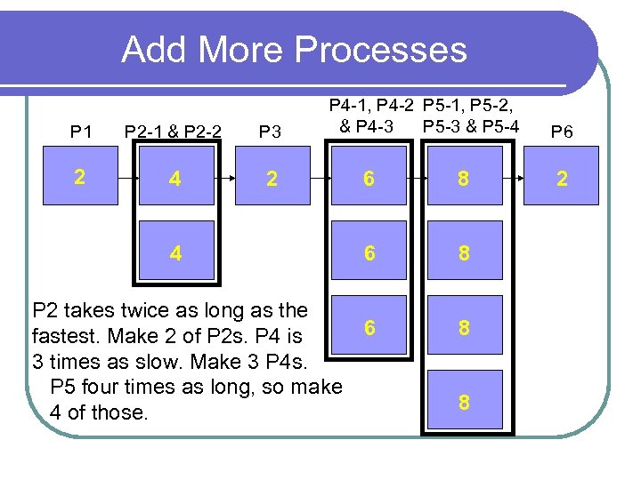Add More Processes P 1 P 2 -1 & P 2 -2 P 3 2 4 P 4 -1, P 4 -2 P 5 -1, P 5 -2, & P 4 -3 P 5 -3 & P 5 -4 2 4 P 2 takes twice as long as the fastest. Make 2 of P 2 s. P 4 is 3 times as slow. Make 3 P 4 s. P 5 four times as long, so make 4 of those. 6 8 6 8 8 P 6 2

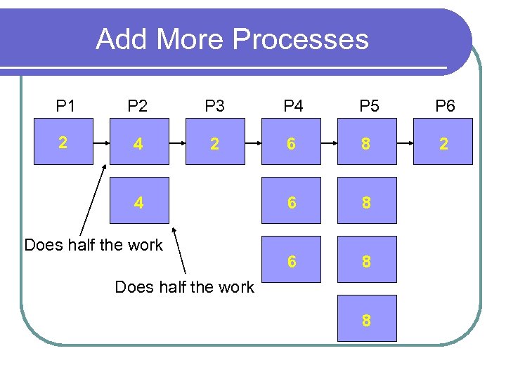Add More Processes P 1 P 2 P 3 P 4 P 5 P 6 2 4 2 6 8 6 8 4 Does half the work 8

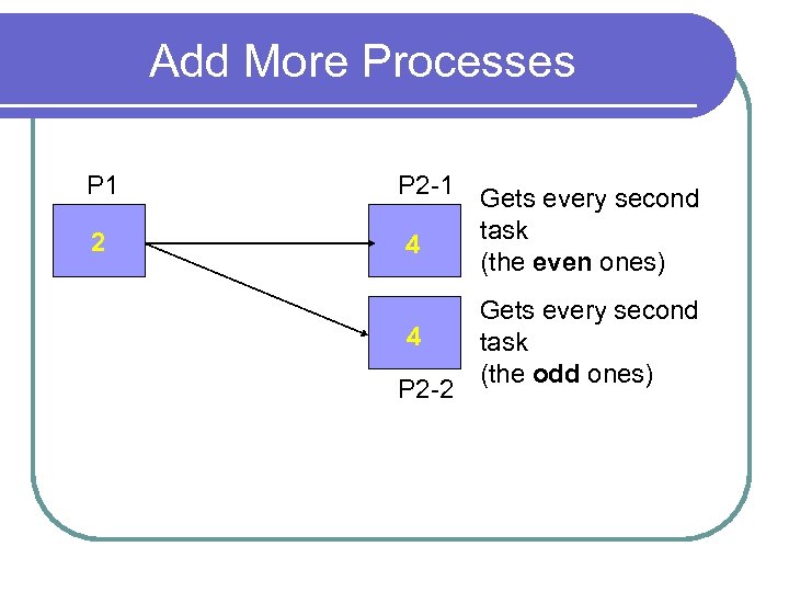Add More Processes P 1 P 2 -1 2 4 4 P 2 -2 Gets every second task (the even ones) Gets every second task (the odd ones)

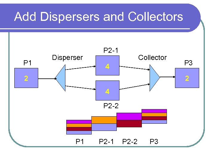Add Dispersers and Collectors P 1 Disperser P 2 -1 Collector 4 2 P 3 2 4 P 2 -2 P 1 P 2 -2 P 3

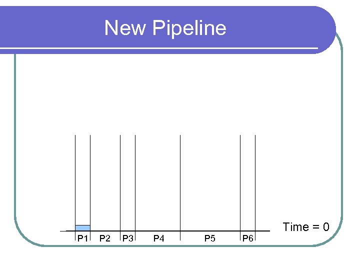New Pipeline P 1 P 2 P 3 P 4 P 5 P 6 Time = 0

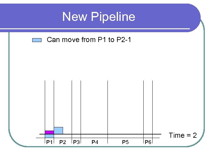New Pipeline Can move from P 1 to P 2 -1 P 2 P 3 P 4 P 5 P 6 Time = 2

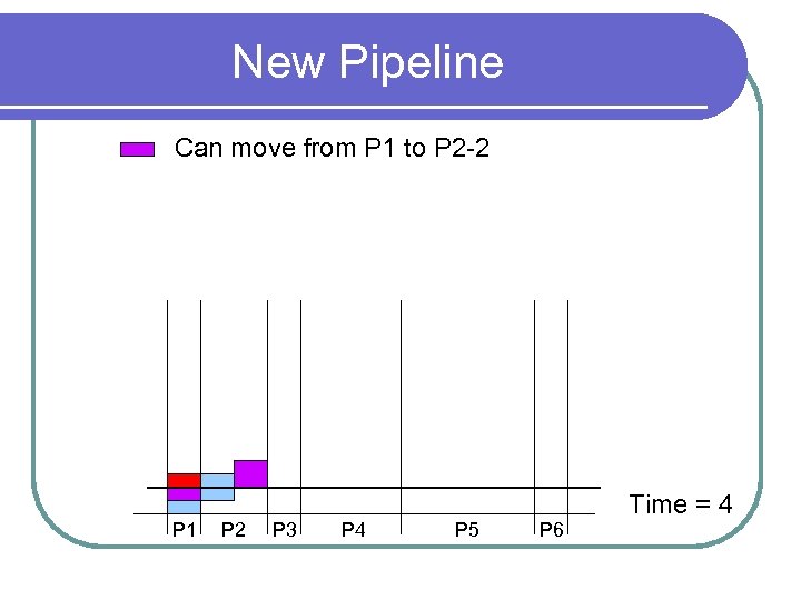New Pipeline Can move from P 1 to P 2 -2 P 1 P 2 P 3 P 4 P 5 P 6 Time = 4

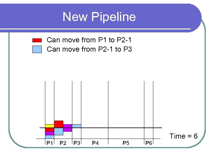New Pipeline Can move from P 1 to P 2 -1 Can move from P 2 -1 to P 3 P 1 P 2 P 3 P 4 P 5 P 6 Time = 6

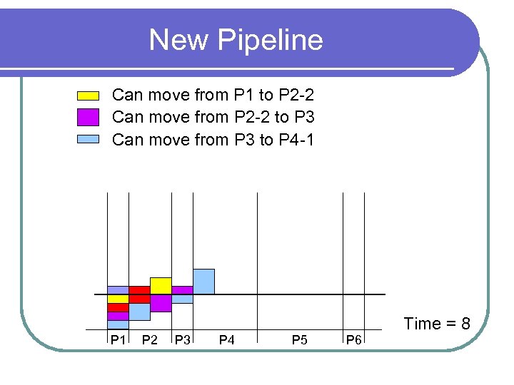New Pipeline Can move from P 1 to P 2 -2 Can move from P 2 -2 to P 3 Can move from P 3 to P 4 -1 P 2 P 3 P 4 P 5 P 6 Time = 8

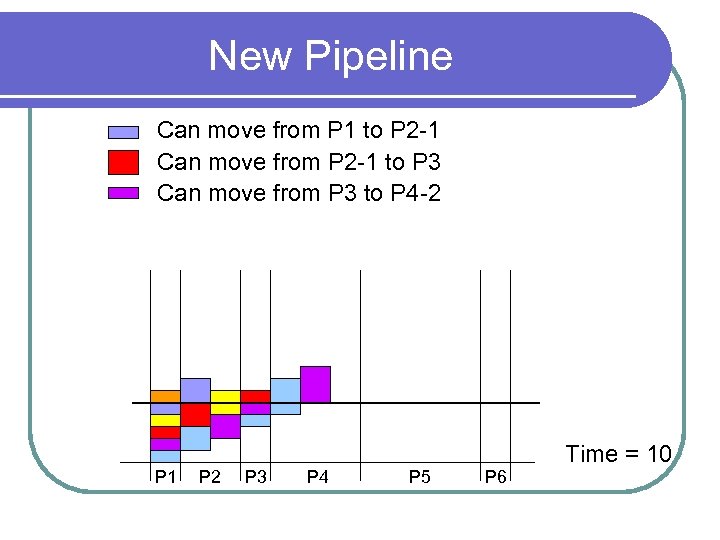New Pipeline Can move from P 1 to P 2 -1 Can move from P 2 -1 to P 3 Can move from P 3 to P 4 -2 P 1 P 2 P 3 P 4 P 5 P 6 Time = 10

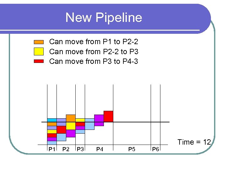New Pipeline Can move from P 1 to P 2 -2 Can move from P 2 -2 to P 3 Can move from P 3 to P 4 -3 P 1 P 2 P 3 P 4 P 5 P 6 Time = 12

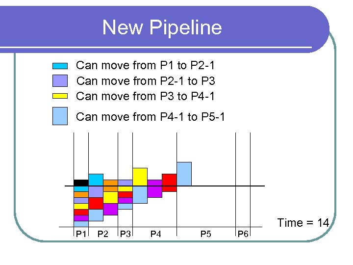New Pipeline Can move from P 1 to P 2 -1 Can move from P 2 -1 to P 3 Can move from P 3 to P 4 -1 Can move from P 4 -1 to P 5 -1 P 2 P 3 P 4 P 5 P 6 Time = 14

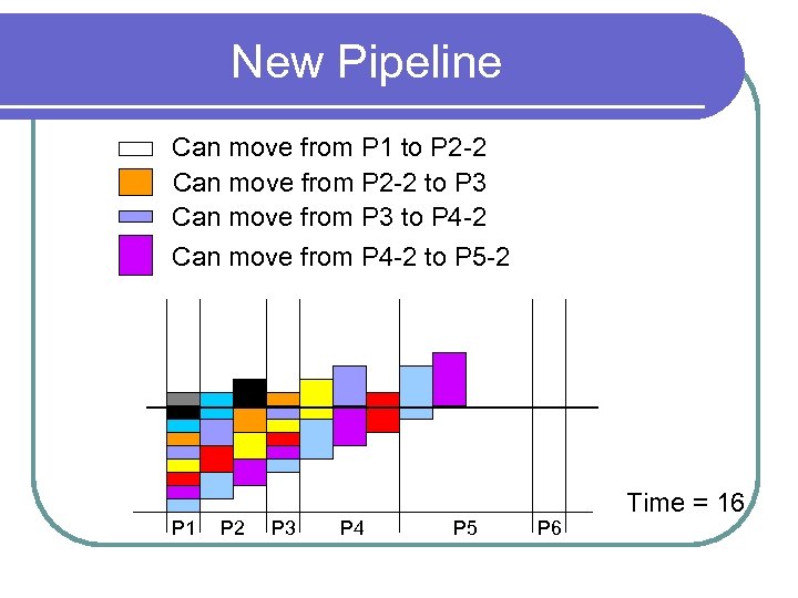New Pipeline Can move from P 1 to P 2 -2 Can move from P 2 -2 to P 3 Can move from P 3 to P 4 -2 Can move from P 4 -2 to P 5 -2 P 1 P 2 P 3 P 4 P 5 P 6 Time = 16

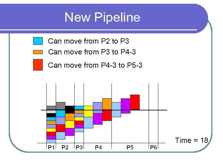New Pipeline Can move from P 2 to P 3 Can move from P 3 to P 4 -3 Can move from P 4 -3 to P 5 -3 P 1 P 2 P 3 P 4 P 5 P 6 Time = 18

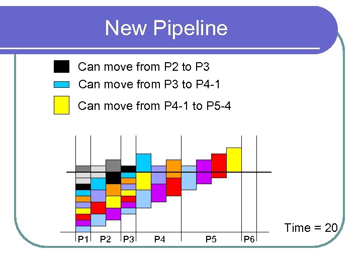New Pipeline Can move from P 2 to P 3 Can move from P 3 to P 4 -1 Can move from P 4 -1 to P 5 -4 P 1 P 2 P 3 P 4 P 5 P 6 Time = 20

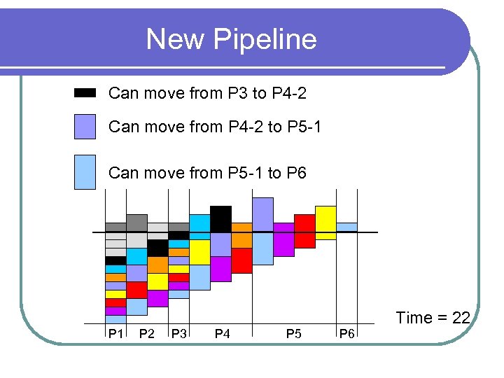New Pipeline Can move from P 3 to P 4 -2 Can move from P 4 -2 to P 5 -1 Can move from P 5 -1 to P 6 P 1 P 2 P 3 P 4 P 5 P 6 Time = 22

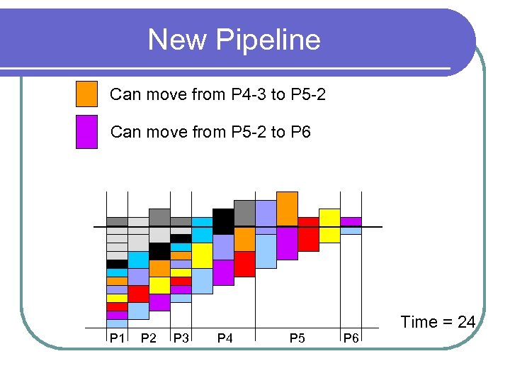New Pipeline Can move from P 4 -3 to P 5 -2 Can move from P 5 -2 to P 6 P 1 P 2 P 3 P 4 P 5 P 6 Time = 24

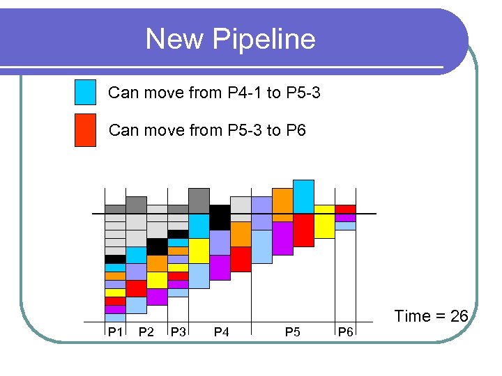New Pipeline Can move from P 4 -1 to P 5 -3 Can move from P 5 -3 to P 6 P 1 P 2 P 3 P 4 P 5 P 6 Time = 26

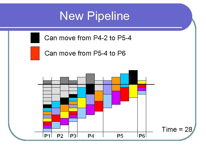New Pipeline Can move from P 4 -2 to P 5 -4 Can move from P 5 -4 to P 6 P 1 P 2 P 3 P 4 P 5 P 6 Time = 28

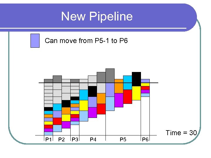New Pipeline Can move from P 5 -1 to P 6 P 1 P 2 P 3 P 4 P 5 P 6 Time = 30

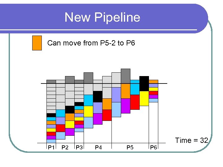New Pipeline Can move from P 5 -2 to P 6 P 1 P 2 P 3 P 4 P 5 P 6 Time = 32

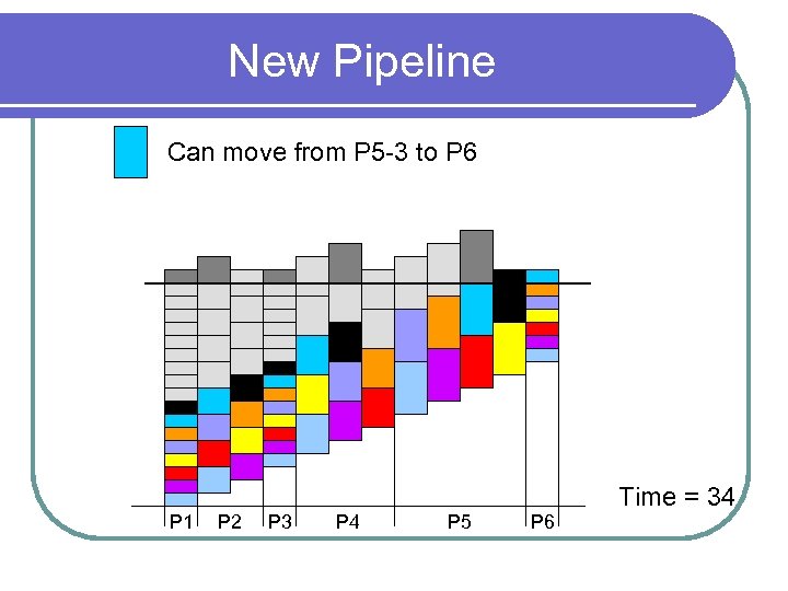New Pipeline Can move from P 5 -3 to P 6 P 1 P 2 P 3 P 4 P 5 P 6 Time = 34

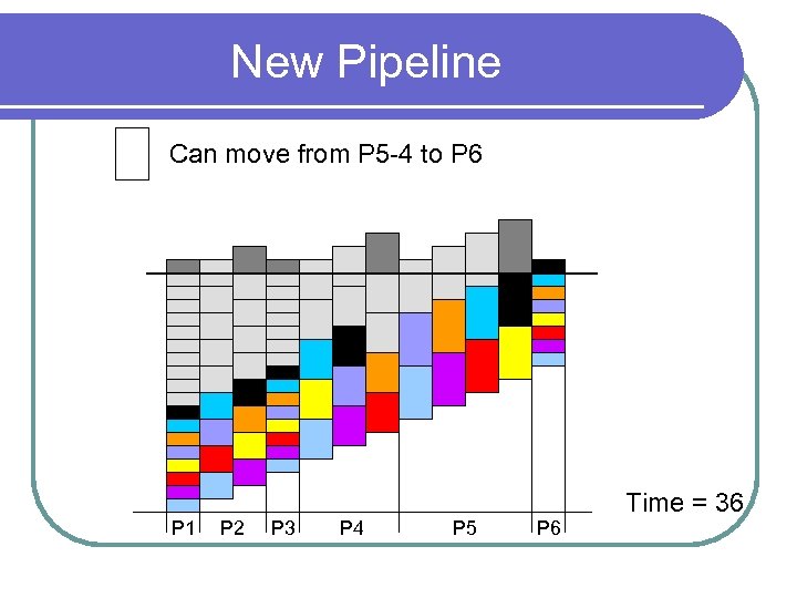New Pipeline Can move from P 5 -4 to P 6 P 1 P 2 P 3 P 4 P 5 P 6 Time = 36

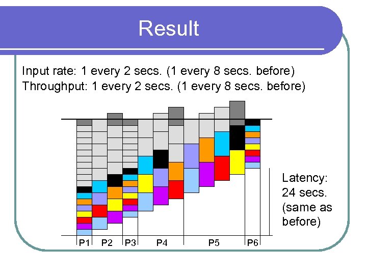Result Input rate: 1 every 2 secs. (1 every 8 secs. before) Throughput: 1 every 2 secs. (1 every 8 secs. before) Latency: 24 secs. (same as before) P 1 P 2 P 3 P 4 P 5 P 6

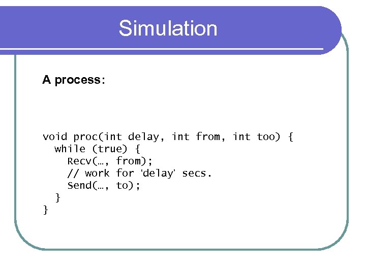Simulation A process: void proc(int delay, int from, int too) { while (true) { Recv(…, from); // work for ‘delay’ secs. Send(…, to); } }

Simulation A disperser: void disperser(int no. Proc, int from, int procs[]) { while (true) { for (i=0; i

Simulation A collector: void collector(int no. Proc, int procs[], int to) { while (true) { for (i=0; i

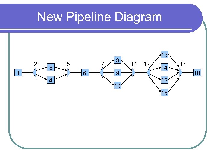New Pipeline Diagram 2 1 3 4 5 7 6 8 9 10 13 11 12 14 15 16 17 18

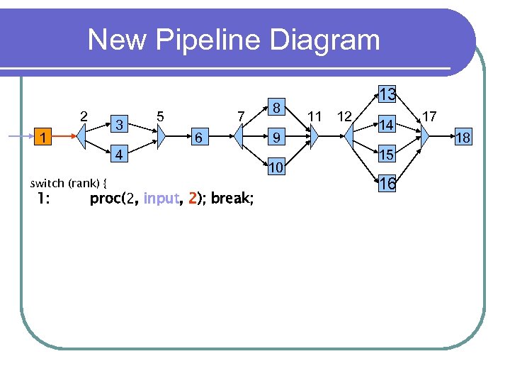New Pipeline Diagram 2 3 1 5 7 6 4 switch (rank) { 1: proc(2, input, 2); break; 8 9 10 13 11 12 14 15 16 17 18

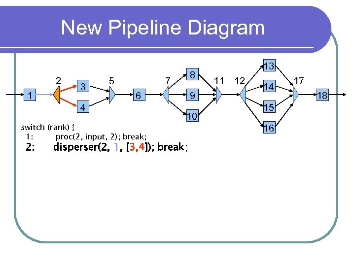New Pipeline Diagram 2 1 3 5 6 4 switch (rank) { 1: proc(2, input, 2); break; 2: 8 7 9 10 disperser(2, 1, [3, 4]); break; 13 11 12 14 15 16 17 18

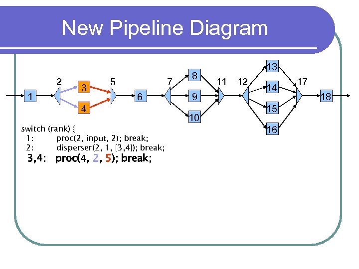New Pipeline Diagram 2 1 3 5 7 6 4 switch (rank) { 1: proc(2, input, 2); break; 2: disperser(2, 1, [3, 4]); break; 3, 4: proc(4, 2, 5); break; 8 9 10 13 11 12 14 15 16 17 18

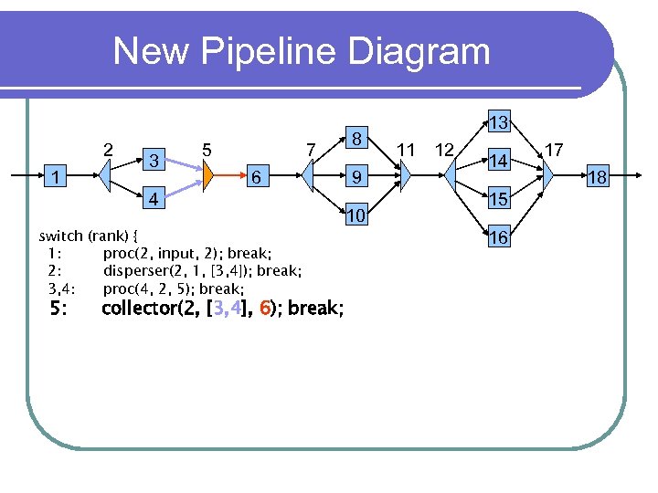New Pipeline Diagram 2 1 3 5 7 6 4 switch (rank) { 1: proc(2, input, 2); break; 2: disperser(2, 1, [3, 4]); break; 3, 4: proc(4, 2, 5); break; 5: collector(2, [3, 4], 6); break; 8 9 10 13 11 12 14 15 16 17 18

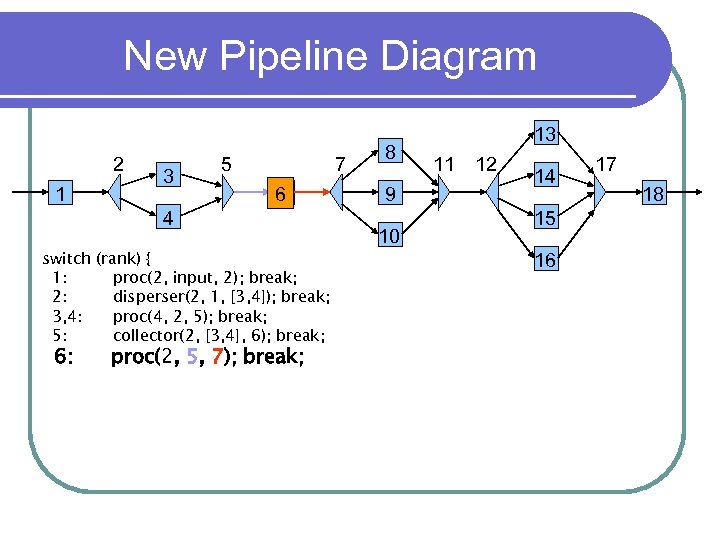New Pipeline Diagram 2 1 3 5 7 6 4 switch (rank) { 1: proc(2, input, 2); break; 2: disperser(2, 1, [3, 4]); break; 3, 4: proc(4, 2, 5); break; 5: collector(2, [3, 4], 6); break; 6: proc(2, 5, 7); break; 8 9 10 13 11 12 14 15 16 17 18

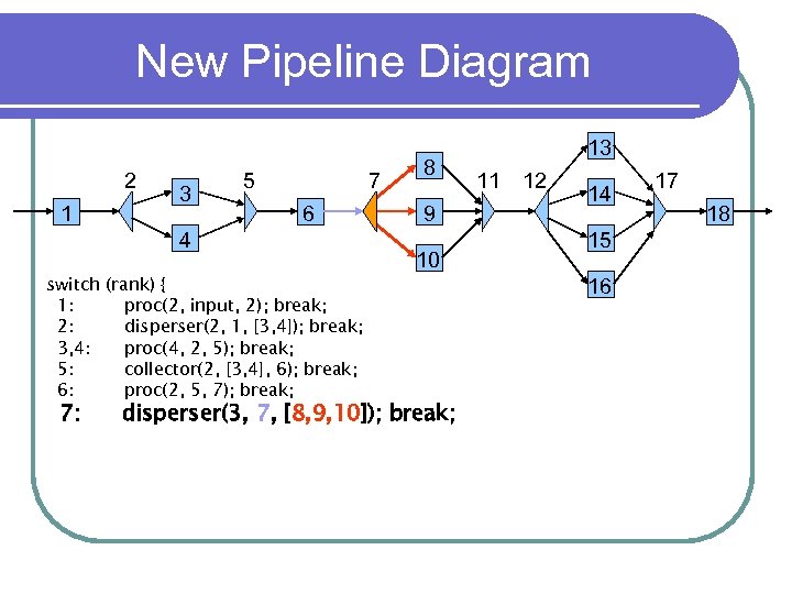New Pipeline Diagram 2 1 3 5 7 6 4 switch (rank) { 1: proc(2, input, 2); break; 2: disperser(2, 1, [3, 4]); break; 3, 4: proc(4, 2, 5); break; 5: collector(2, [3, 4], 6); break; 6: proc(2, 5, 7); break; 7: 8 9 10 disperser(3, 7, [8, 9, 10]); break; 13 11 12 14 15 16 17 18

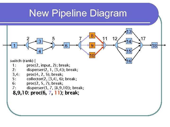New Pipeline Diagram 2 1 3 5 7 6 4 switch (rank) { 1: proc(2, input, 2); break; 2: disperser(2, 1, [3, 4]); break; 3, 4: proc(4, 2, 5); break; 5: collector(2, [3, 4], 6); break; 6: proc(2, 5, 7); break; 7: disperser(3, 7, [8, 9, 10]); break; 8, 9, 10: proc(6, 7, 11); break; 8 9 10 13 11 12 14 15 16 17 18

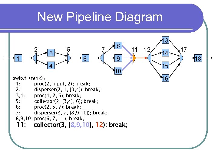New Pipeline Diagram 2 1 3 5 7 6 4 switch (rank) { 1: proc(2, input, 2); break; 2: disperser(2, 1, [3, 4]); break; 3, 4: proc(4, 2, 5); break; 5: collector(2, [3, 4], 6); break; 6: proc(2, 5, 7); break; 7: disperser(3, 7, [8, 9, 10]); break; 8, 9, 10: proc(6, 7, 11); break; 11: 8 9 10 collector(3, [8, 9, 10], 12); break; 13 11 12 14 15 16 17 18

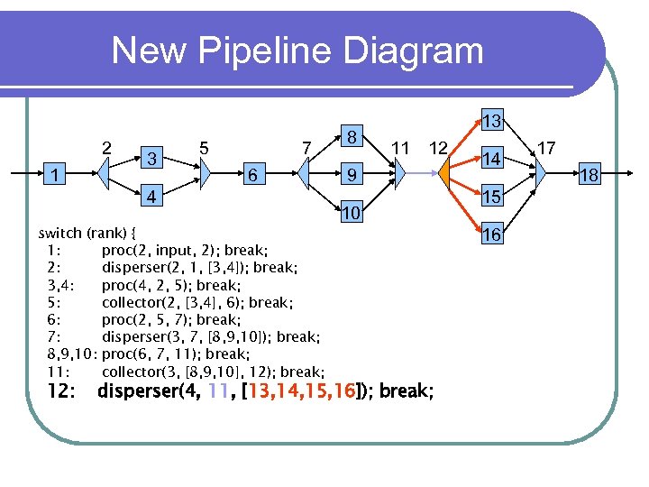New Pipeline Diagram 2 1 3 5 7 6 4 switch (rank) { 1: proc(2, input, 2); break; 2: disperser(2, 1, [3, 4]); break; 3, 4: proc(4, 2, 5); break; 5: collector(2, [3, 4], 6); break; 6: proc(2, 5, 7); break; 7: disperser(3, 7, [8, 9, 10]); break; 8, 9, 10: proc(6, 7, 11); break; 11: collector(3, [8, 9, 10], 12); break; 12: 8 13 11 12 9 10 disperser(4, 11, [13, 14, 15, 16]); break; 14 15 16 17 18

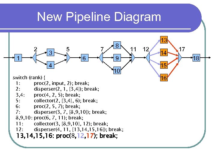New Pipeline Diagram 2 1 3 4 5 7 6 8 9 10 switch (rank) { 1: proc(2, input, 2); break; 2: disperser(2, 1, [3, 4]); break; 3, 4: proc(4, 2, 5); break; 5: collector(2, [3, 4], 6); break; 6: proc(2, 5, 7); break; 7: disperser(3, 7, [8, 9, 10]); break; 8, 9, 10: proc(6, 7, 11); break; 11: collector(3, [8, 9, 10], 12); break; 12: disperser(4, 11, [13, 14, 15, 16]); break; 13, 14, 15, 16: proc(8, 12, 17); break; 13 11 12 14 15 16 17 18

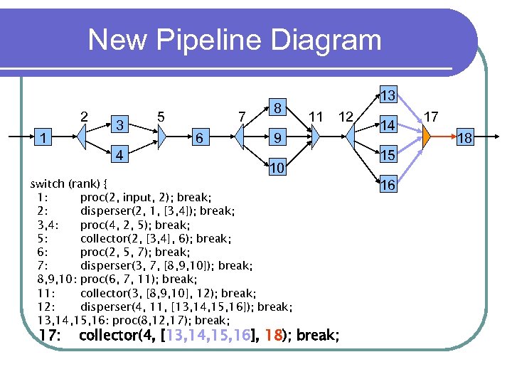New Pipeline Diagram 2 1 3 4 5 7 6 8 11 12 9 10 switch (rank) { 1: proc(2, input, 2); break; 2: disperser(2, 1, [3, 4]); break; 3, 4: proc(4, 2, 5); break; 5: collector(2, [3, 4], 6); break; 6: proc(2, 5, 7); break; 7: disperser(3, 7, [8, 9, 10]); break; 8, 9, 10: proc(6, 7, 11); break; 11: collector(3, [8, 9, 10], 12); break; 12: disperser(4, 11, [13, 14, 15, 16]); break; 13, 14, 15, 16: proc(8, 12, 17); break; 17: 13 collector(4, [13, 14, 15, 16], 18); break; 14 15 16 17 18

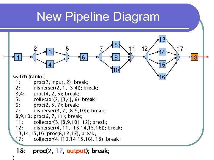New Pipeline Diagram 2 1 3 5 7 6 4 8 9 10 switch (rank) { 1: proc(2, input, 2); break; 2: disperser(2, 1, [3, 4]); break; 3, 4: proc(4, 2, 5); break; 5: collector(2, [3, 4], 6); break; 6: proc(2, 5, 7); break; 7: disperser(3, 7, [8, 9, 10]); break; 8, 9, 10: proc(6, 7, 11); break; 11: collector(3, [8, 9, 10], 12); break; 12: disperser(4, 11, [13, 14, 15, 16]); break; 13, 14, 15, 16: proc(8, 12, 17); break; 17: collector(4, [13, 14, 15, 16], 18); break; } 18: proc(2, 17, output); break; 13 11 12 14 15 16 17 18

Improvement ? l Theory: l We went from 1 packet every 8 seconds to 1 every 2 seconds l Practice: l Run the program and see

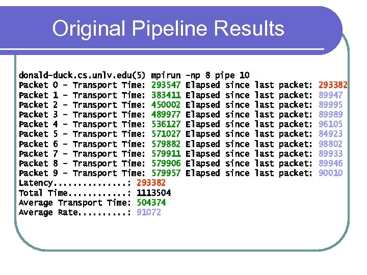Original Pipeline Results donald-duck. cs. unlv. edu(5) mpirun Packet 0 - Transport Time: 293547 Packet 1 - Transport Time: 383411 Packet 2 - Transport Time: 450002 Packet 3 - Transport Time: 489977 Packet 4 - Transport Time: 536127 Packet 5 - Transport Time: 571027 Packet 6 - Transport Time: 579882 Packet 7 - Transport Time: 579911 Packet 8 - Transport Time: 579906 Packet 9 - Transport Time: 579957 Latency. . . . : 293382 Total Time. . . : 1113504 Average Transport Time: 504374 Average Rate. . : 91072 -np 8 pipe 10 Elapsed since Elapsed since Elapsed since last last last packet: packet: packet: 293382 89947 89995 89989 96105 84923 98802 89933 89946 90010

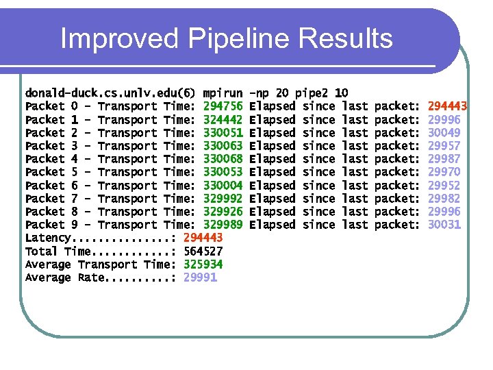Improved Pipeline Results donald-duck. cs. unlv. edu(6) mpirun Packet 0 - Transport Time: 294756 Packet 1 - Transport Time: 324442 Packet 2 - Transport Time: 330051 Packet 3 - Transport Time: 330063 Packet 4 - Transport Time: 330068 Packet 5 - Transport Time: 330053 Packet 6 - Transport Time: 330004 Packet 7 - Transport Time: 329992 Packet 8 - Transport Time: 329926 Packet 9 - Transport Time: 329989 Latency. . . . : 294443 Total Time. . . : 564527 Average Transport Time: 325934 Average Rate. . : 29991 -np 20 pipe 2 10 Elapsed since last Elapsed since last Elapsed since last packet: packet: packet: 294443 29996 30049 29957 29987 29970 29952 29982 29996 30031

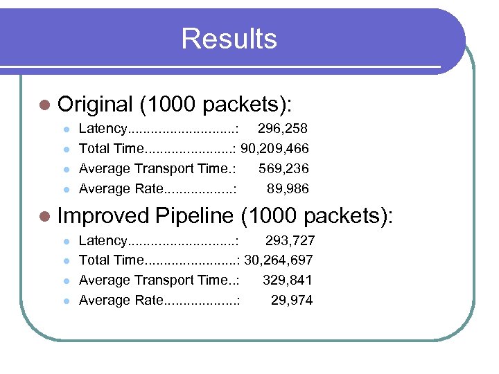Results l Original l l (1000 packets): Latency. . . . : 296, 258 Total Time. . . : 90, 209, 466 Average Transport Time. : 569, 236 Average Rate. . . . : 89, 986 l Improved l l Pipeline (1000 packets): Latency. . . . : 293, 727 Total Time. . . : 30, 264, 697 Average Transport Time. . : 329, 841 Average Rate. . . . . : 29, 974

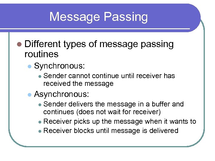Message Passing l Different routines l Synchronous: l l types of message passing Sender cannot continue until receiver has received the message Asynchronous: Sender delivers the message in a buffer and continues (does not wait for receiver) l Receiver picks up the message when it wants to l Receiver blocks until message is delivered l

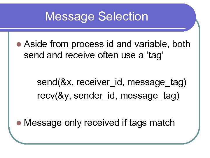Message Selection l Aside from process id and variable, both send and receive often use a ‘tag’ send(&x, receiver_id, message_tag) recv(&y, sender_id, message_tag) l Message only received if tags match

Message Passing in MPI l = Message Passing Interface Originally not a product, but a specification l C/C++ & Fortran libraries l Earlier message passing library is PVM = Parallel Virtual Machine

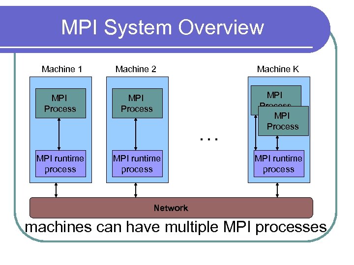MPI System Overview Machine 1 Machine 2 Machine K MPI Process … MPI runtime process Network machines can have multiple MPI processes

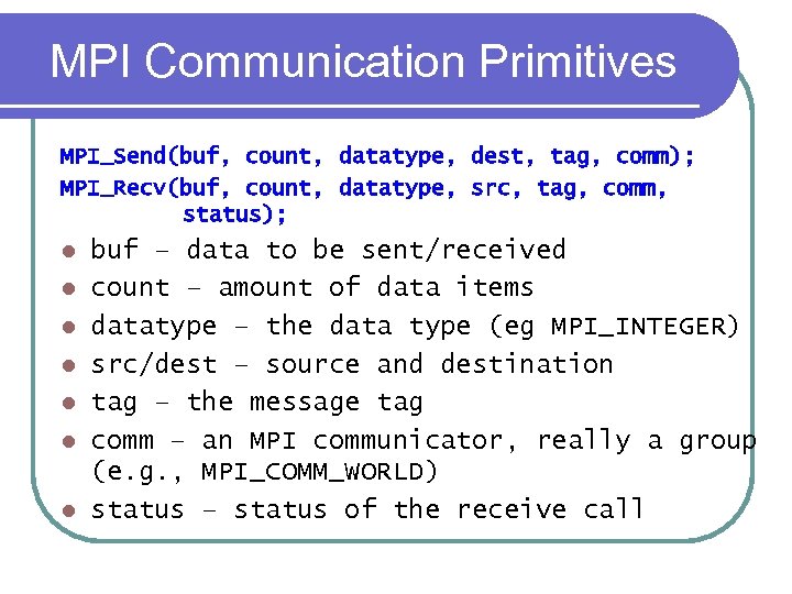MPI Communication Primitives MPI_Send(buf, count, datatype, dest, tag, comm); MPI_Recv(buf, count, datatype, src, tag, comm, status); l l l l buf – data to be sent/received count – amount of data items datatype – the data type (eg MPI_INTEGER) src/dest – source and destination tag – the message tag comm – an MPI communicator, really a group (e. g. , MPI_COMM_WORLD) status – status of the receive call

MPI Program Skeleton Master/slave Skeleton MPI Program: Int main(int argc, char *argv[]) { int rank; MPI_Init(&argc, &argv); MPI_Comm_rank(MPI_COMM_WORLD, &rank); if (myrank == 0) master(); else slave(); } Rank is a process’ ID In the MPI session

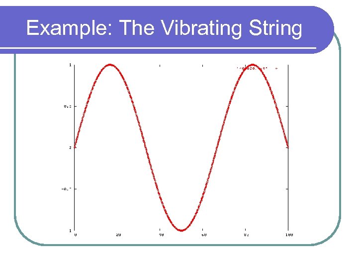Example: The Vibrating String

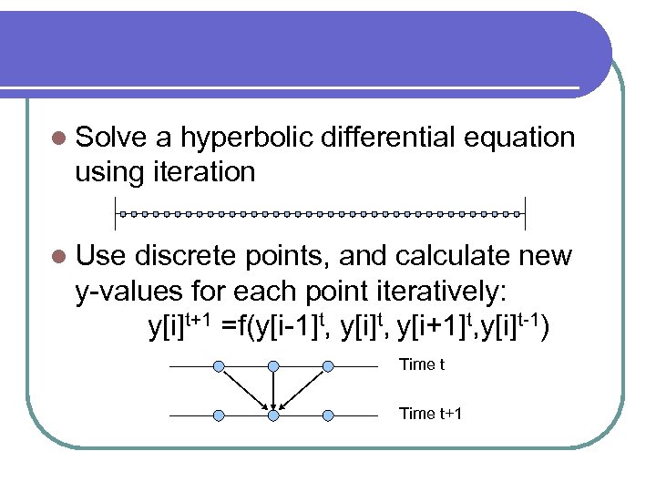l Solve a hyperbolic differential equation using iteration l Use discrete points, and calculate new y-values for each point iteratively: y[i]t+1 =f(y[i-1]t, y[i+1]t, y[i]t-1) Time t+1

l Sequential algorithm: for (s=0; s

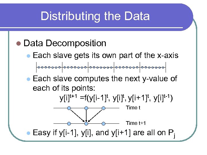Distributing the Data l Data Decomposition l Each slave gets its own part of the x-axis l Each slave computes the next y-value of each of its points: y[i]t+1 =f(y[i-1]t, y[i+1]t, y[i]t-1) Time t+1 l Easy if y[i-1], y[i], and y[i+1] are all on Pj

Data Distribution and Communication l What if, say y[i-1], is on Pj-1 and y[i] and y[i+1] are on Pj? Time t+1 Pj-1 l Pj-1 Pj and Pj must exchange values by communicating

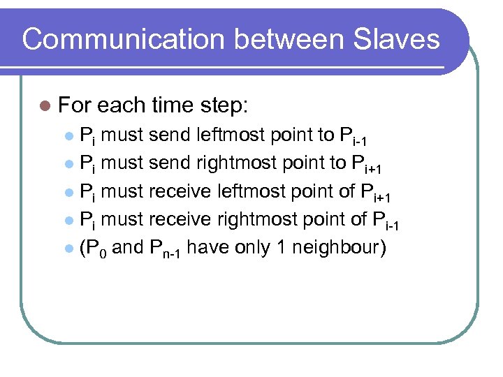Communication between Slaves l For each time step: Pi must send leftmost point to Pi-1 l Pi must send rightmost point to Pi+1 l Pi must receive leftmost point of Pi+1 l Pi must receive rightmost point of Pi-1 l (P 0 and Pn-1 have only 1 neighbour) l

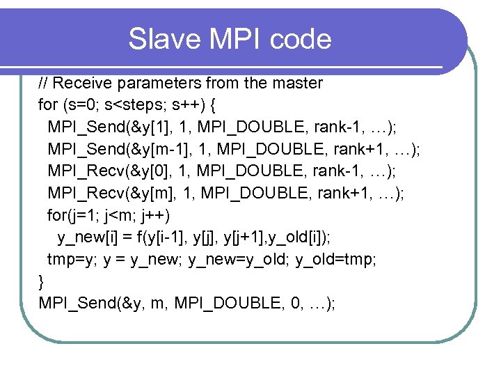Slave MPI code // Receive parameters from the master for (s=0; s

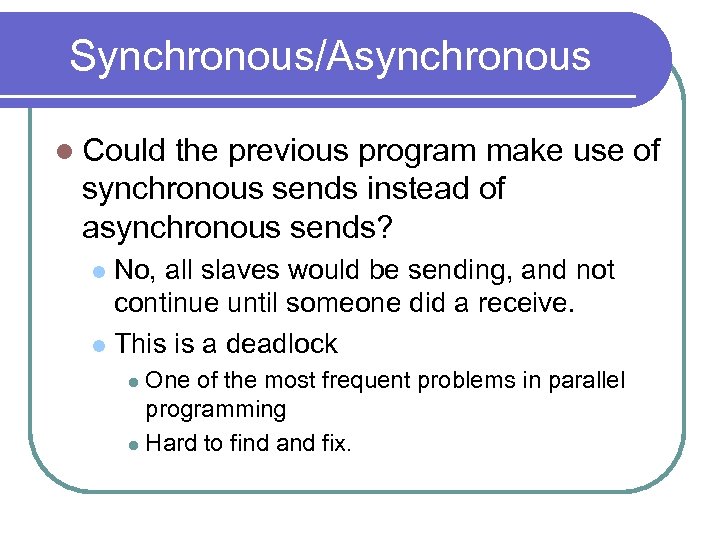Synchronous/Asynchronous l Could the previous program make use of synchronous sends instead of asynchronous sends? No, all slaves would be sending, and not continue until someone did a receive. l This is a deadlock l One of the most frequent problems in parallel programming l Hard to find and fix. l

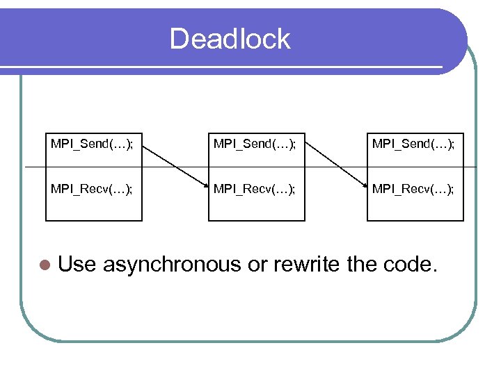Deadlock MPI_Send(…); MPI_Recv(…); l Use asynchronous or rewrite the code.

Load Balancing l “Load” = The amount of work for a process(or) l Mandelbrot Each slave gets the same number of points l Should be nicely load balanced l Black pixels take longer l What if one slave got 2 times as many black pixels than any other? l

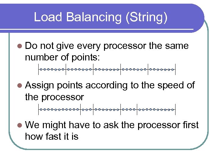
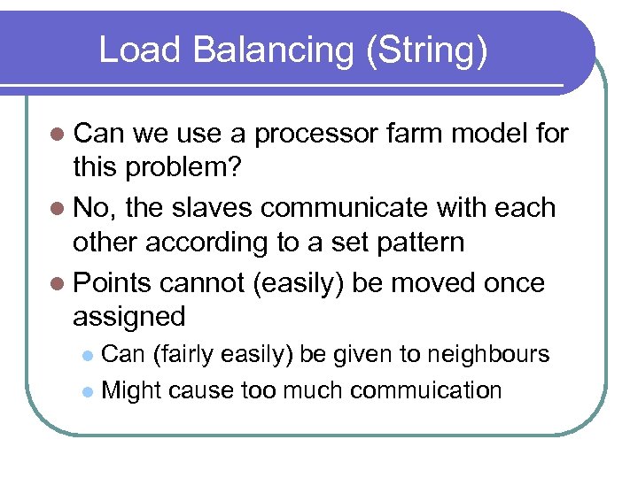
Load Balancing l Vibrating String Each slave gets the same number of points l This SHOULD be nicely load balanced l l l Each point takes the same amount of time What if one machine is simply slower than the others?

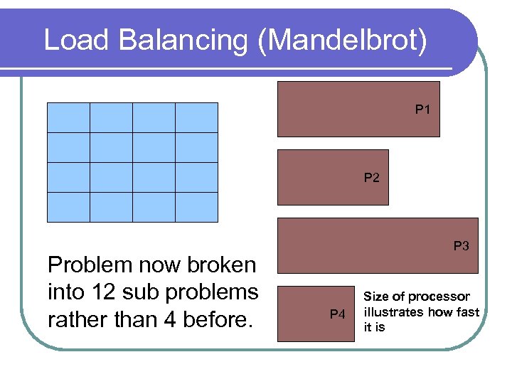
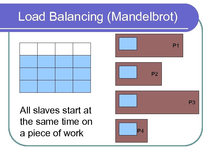
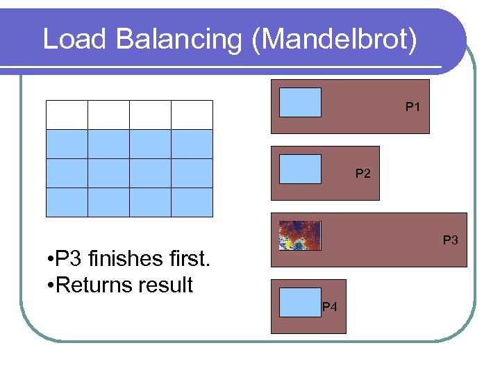
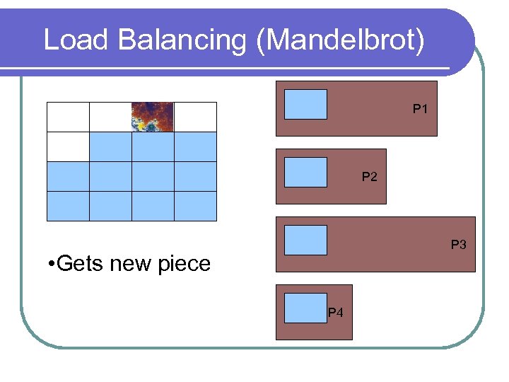
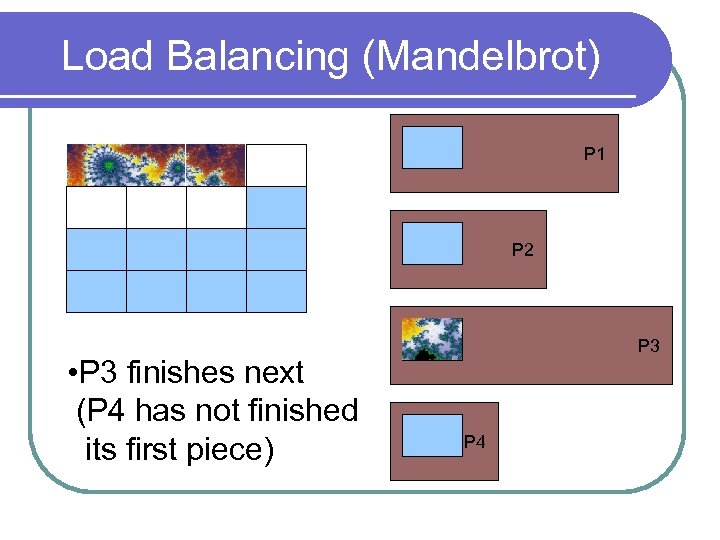
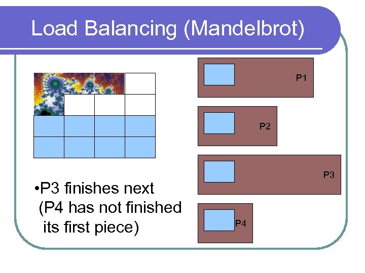
Load Balancing (Mandelbrot) l There is no way to know how many points turn into black pixels without doing the computation. l Solution Don’t divide problem into n=p pieces. l Divide it into m > p pieces l

Load Balancing (Mandelbrot) l Use a technique called ‘Processor Farm’ Each slave is initially given a piece of work l When a slave is done it asks for more work l This way faster slaves work ‘harder’ and slower ones ‘less hard’ l

Load Balancing (Mandelbrot) P 1 P 2 Problem now broken into 12 sub problems rather than 4 before. P 3 P 4 Size of processor illustrates how fast it is

Load Balancing (Mandelbrot) P 1 P 2 All slaves start at the same time on a piece of work P 3 P 4

Load Balancing (Mandelbrot) P 1 P 2 P 3 • P 3 finishes first. • Returns result P 4

Load Balancing (Mandelbrot) P 1 P 2 P 3 • Gets new piece P 4

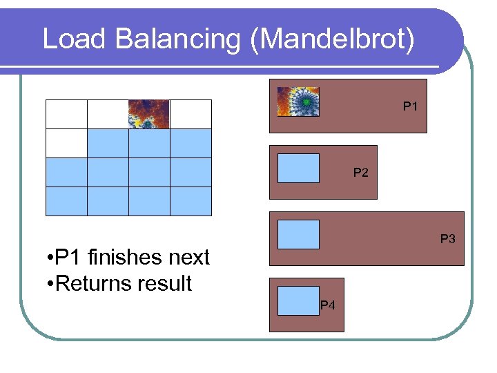Load Balancing (Mandelbrot) P 1 P 2 P 3 • P 1 finishes next • Returns result P 4

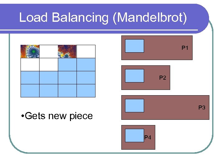Load Balancing (Mandelbrot) P 1 P 2 P 3 • Gets new piece P 4

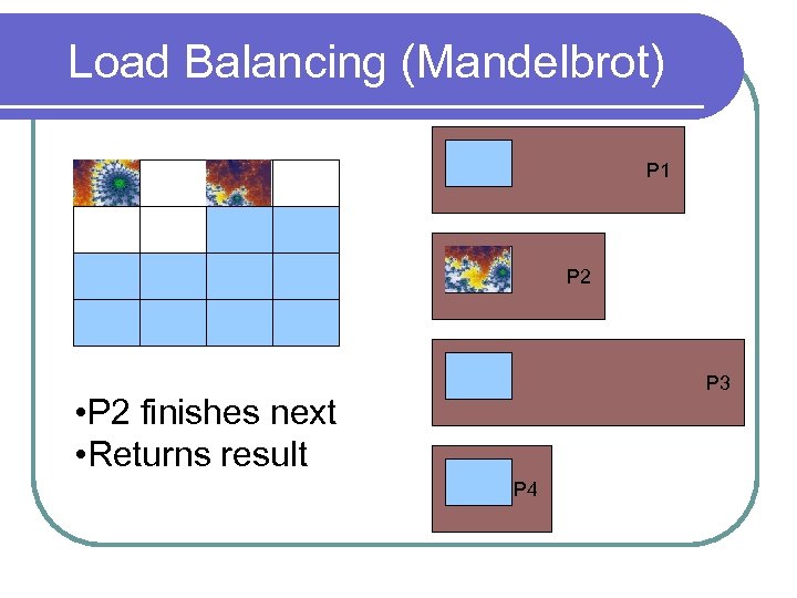Load Balancing (Mandelbrot) P 1 P 2 P 3 • P 2 finishes next • Returns result P 4

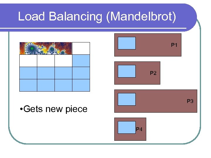Load Balancing (Mandelbrot) P 1 P 2 P 3 • Gets new piece P 4

Load Balancing (Mandelbrot) P 1 P 2 • P 3 finishes next (P 4 has not finished its first piece) P 3 P 4

Load Balancing (Mandelbrot) P 1 P 2 • P 3 finishes next (P 4 has not finished its first piece) P 3 P 4

Load Balancing (String) l Do not give every processor the same number of points: l Assign points according to the speed of the processor l We might have to ask the processor first how fast it is

Load Balancing (String) l Can we use a processor farm model for this problem? l No, the slaves communicate with each other according to a set pattern l Points cannot (easily) be moved once assigned Can (fairly easily) be given to neighbours l Might cause too much commuication l

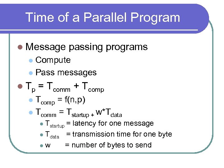Time of a Parallel Program l Message passing programs Compute l Pass messages l l Tp = Tcomm + Tcomp = f(n, p) l Tcomm = Tstartup + w*Tdata l Tstartup = latency for one message l Tdata = transmission time for one byte lw = number of bytes to send l

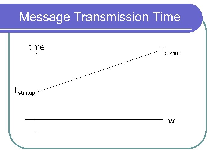Message Transmission Time time Tcomm Tstartup w

Should We Buy an Earth Simulator? l How many processors should we use? As few as possible? l As many as possible? l l Can be hard to answer l Example: Solving a system of linear equations using iteration

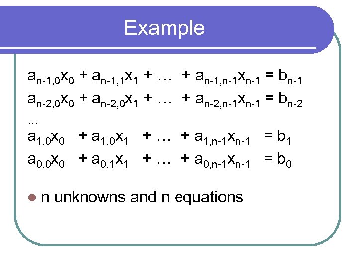Example an-1, 0 x 0 + an-1, 1 x 1 + … + an-1, n-1 xn-1 = bn-1 an-2, 0 x 0 + an-2, 0 x 1 + … + an-2, n-1 xn-1 = bn-2 … a 1, 0 x 0 + a 1, 0 x 1 + … + a 1, n-1 xn-1 = b 1 a 0, 0 x 0 + a 0, 1 x 1 + … + a 0, n-1 xn-1 = b 0 ln unknowns and n equations

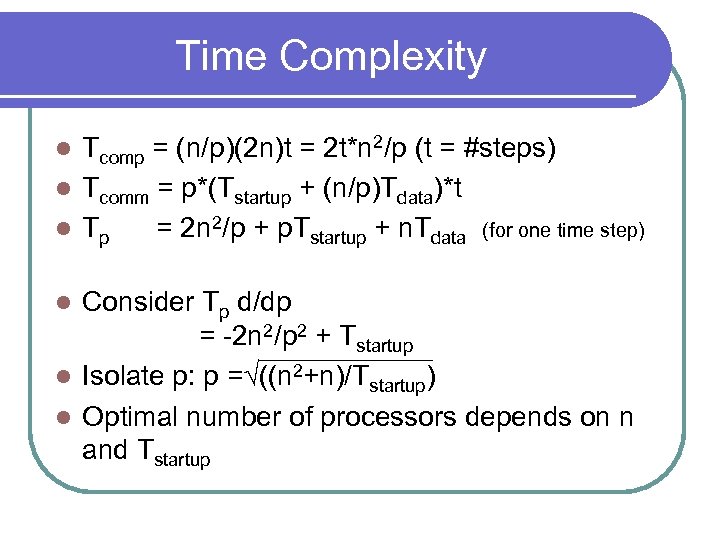Time Complexity Tcomp = (n/p)(2 n)t = 2 t*n 2/p (t = #steps) l Tcomm = p*(Tstartup + (n/p)Tdata)*t l Tp = 2 n 2/p + p. Tstartup + n. Tdata (for one time step) l Consider Tp d/dp = -2 n 2/p 2 + Tstartup l Isolate p: p =√((n 2+n)/Tstartup) l Optimal number of processors depends on n and Tstartup l

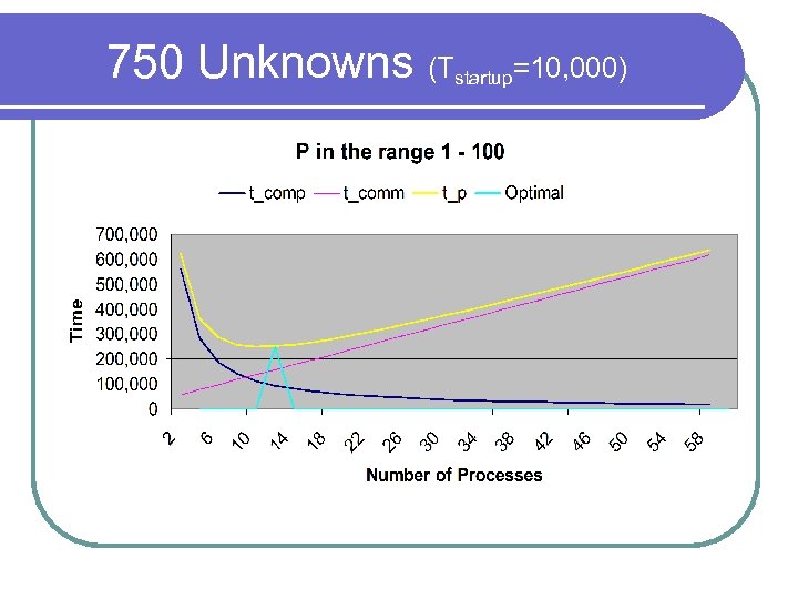750 Unknowns (Tstartup=10, 000)

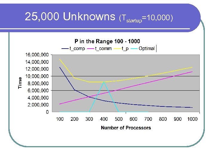25, 000 Unknowns (Tstartup=10, 000)

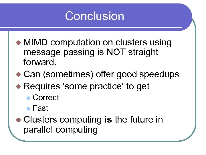Conclusion l MIMD computation on clusters using message passing is NOT straight forward. l Can (sometimes) offer good speedups l Requires ‘some practice’ to get Correct l Fast l l Clusters computing is the future in parallel computing

Note l This material is available at http: //www. cs. unlv. edu/~matt under ‘research’ l Email: matt@cs. unlv. edu