9ec3f5ac9e4841b83d44a52f08cecdf7.ppt
- Количество слайдов: 45
CPT-S 580 -06 Advanced Databases Yinghui Wu EME 49 1
Query processing over large datasets 2
Querying Big Data: Theory and Practice ü Theory – Tractability revisited for querying big data – Parallel scalability – Bounded evaluability ü Techniques – Approximate query processing – Parallel algorithms – Bounded evaluability and access constraints – Query-preserving compression – Query answering using views – Bounded incremental query processing 3
Fundamental question To query big data, we have to determine whether it is feasible at all. For a class Q of queries, can we find an algorithm T such that given any Q in Q and any big dataset D, T efficiently computes the answers Q(D) of Q in D within our available resources? Is this feasible or not for Q? ü Tractability revised for querying big data (BD-tractability) ü Parallel scalability (in future lecture) ü Bounded evaluability (in future lecture) New theory for querying big data 4
A review of P, NP and intractability 5
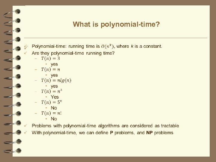
What is polynomial-time? ü
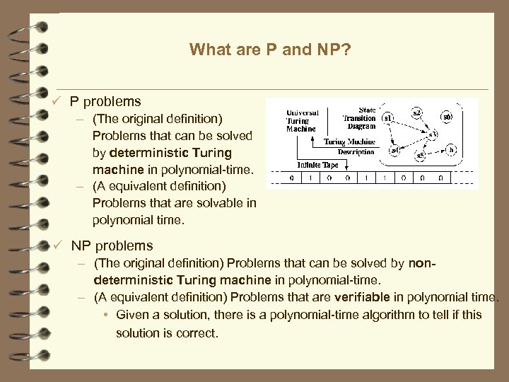
What are P and NP? ü P problems – (The original definition) Problems that can be solved by deterministic Turing machine in polynomial-time. – (A equivalent definition) Problems that are solvable in polynomial time. ü NP problems – (The original definition) Problems that can be solved by nondeterministic Turing machine in polynomial-time. – (A equivalent definition) Problems that are verifiable in polynomial time. • Given a solution, there is a polynomial-time algorithm to tell if this solution is correct.
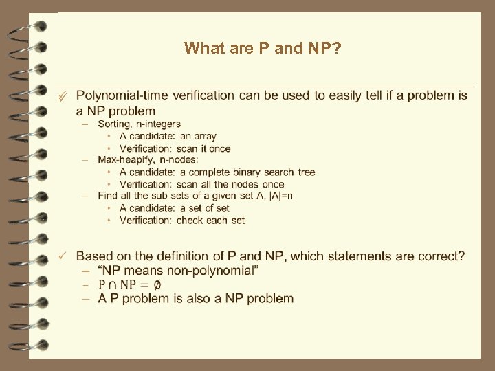
What are P and NP? ü
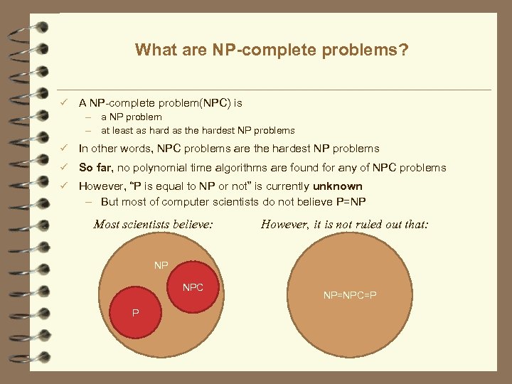
What are NP-complete problems? ü A NP-complete problem(NPC) is – a NP problem – at least as hard as the hardest NP problems ü In other words, NPC problems are the hardest NP problems ü So far, no polynomial time algorithms are found for any of NPC problems ü However, “P is equal to NP or not” is currently unknown – But most of computer scientists do not believe P=NP Most scientists believe: However, it is not ruled out that: NP NPC P NP=NPC=P
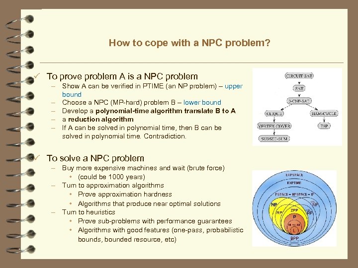
How to cope with a NPC problem? ü To prove problem A is a NPC problem – Show A can be verified in PTIME (an NP problem) – upper bound – Choose a NPC (MP-hard) problem B – lower bound – Develop a polynomial-time algorithm translate B to A – a reduction algorithm – If A can be solved in polynomial time, then B can be solved in polynomial time. Contradiction. ü To solve a NPC problem – Buy more expensive machines and wait (brute force) • (could be 1000 years) – Turn to approximation algorithms • Prove approximation hardness • Algorithms that produce near optimal solutions – Turn to heuristics • Prove sub-problems with performance guarantees • Algorithms with good features (one-pass, probabilistic bounds, bounded resource, etc)
BD-tractability 11
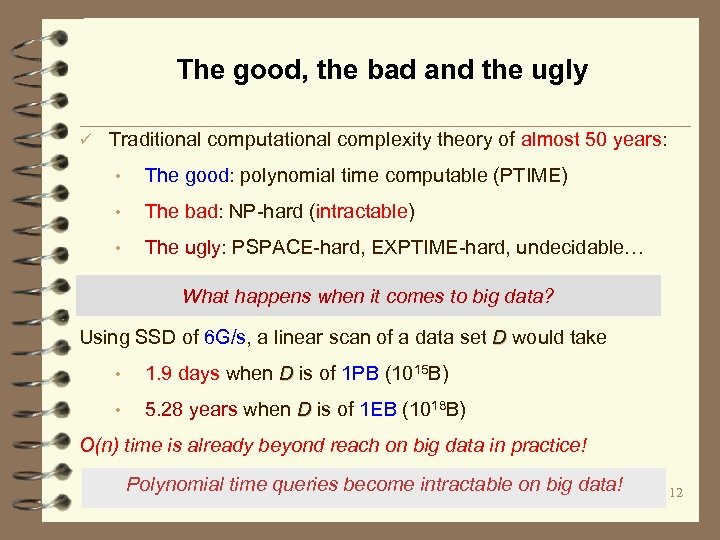
The good, the bad and the ugly ü Traditional computational complexity theory of almost 50 years: • The good: polynomial time computable (PTIME) • The bad: NP-hard (intractable) • The ugly: PSPACE-hard, EXPTIME-hard, undecidable… What happens when it comes to big data? Using SSD of 6 G/s, a linear scan of a data set D would take • 1. 9 days when D is of 1 PB (1015 B) • 5. 28 years when D is of 1 EB (1018 B) O(n) time is already beyond reach on big data in practice! Polynomial time queries become intractable on big data! 12
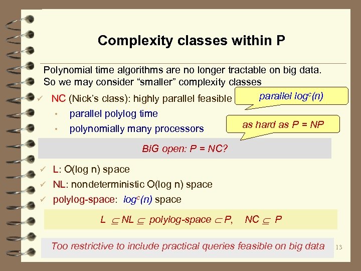
Complexity classes within P Polynomial time algorithms are no longer tractable on big data. So we may consider “smaller” complexity classes parallel logc(n) ü NC (Nick’s class): highly parallel feasible • parallel polylog time • polynomially many processors as hard as P = NP BIG open: P = NC? L: O(log n) space ü NL: nondeterministic O(log n) space ü ü polylog-space: logc(n) space L NL polylog-space P, NC P Too restrictive to include practical queries feasible on big data 13
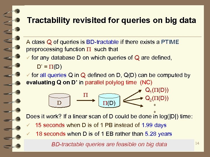
Tractability revisited for queries on big data A class Q of queries is BD-tractable if there exists a PTIME preprocessing function such that ü for any database D on which queries of Q are defined, D’ = (D) ü for all queries Q in Q defined on D, Q(D) can be computed by evaluating Q on D’ in parallel polylog time (NC) Q 1( (D)) Q 2( (D)) D (D) 。 。 Does it work? If a linear scan of D could be done in log(|D|) time: ü 15 seconds when D is of 1 PB instead of 1. 99 days ü 18 seconds when D is of 1 EB rather than 5. 28 years BD-tractable queries are feasible on big data 14
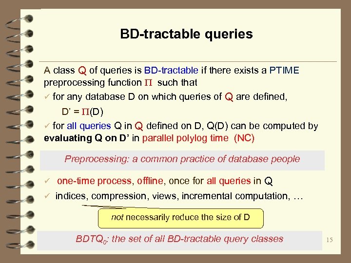
BD-tractable queries A class Q of queries is BD-tractable if there exists a PTIME preprocessing function such that ü for any database D on which queries of Q are defined, D’ = (D) ü for all queries Q in Q defined on D, Q(D) can be computed by evaluating Q on D’ in parallel polylog time (NC) Preprocessing: a common practice of database people ü one-time process, offline, once for all queries in Q ü indices, compression, views, incremental computation, … not necessarily reduce the size of D BDTQ 0: the set of all BD-tractable query classes 15
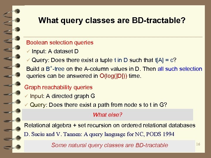
What query classes are BD-tractable? Boolean selection queries ü Input: A dataset D ü Query: Does there exist a tuple t in D such that t[A] = c? Build a B+-tree on the A-column values in D. Then all such selection queries can be answered in O(log(|D|)) time. Graph reachability queries ü Input: A directed graph G ü Query: Does there exist a path from node s to t in G? What else? Relational algebra + set recursion on ordered relational databases D. Suciu and V. Tannen: A query language for NC, PODS 1994 Some natural query classes are BD-tractable 16
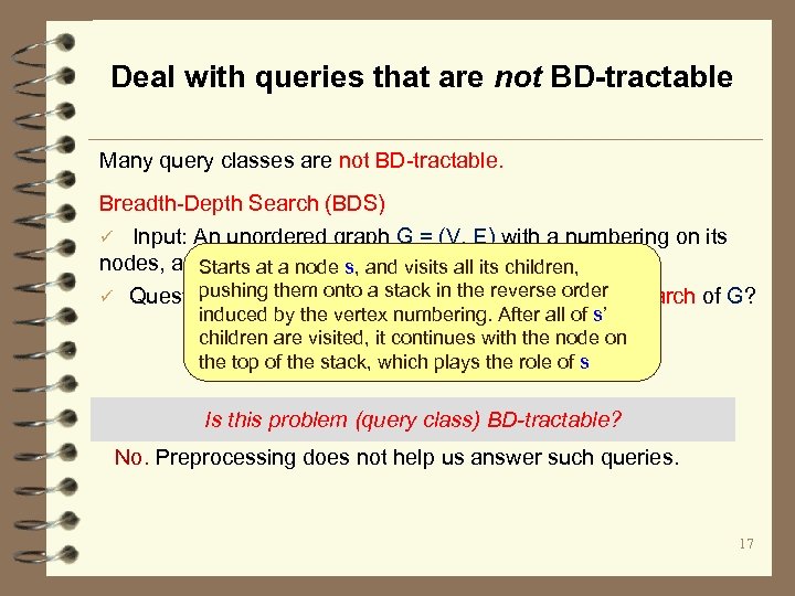
Deal with queries that are not BD-tractable Many query classes are not BD-tractable. Breadth-Depth Search (BDS) ü Input: An unordered graph G = (V, E) with a numbering on its nodes, and a pair (u, v) of nodes in V Starts at a node s, and visits all its children, pushing them onto a stack in the reverse order ü Question: Is u visited before v in the breadth-depth search of G? induced by the vertex numbering. After all of s’ children are visited, it continues with the node on the top of the stack, which plays the role of s Is this problem (query class) BD-tractable? No. Preprocessing does not help us answer such queries. 17
Fundamental problems for BD-tractability BD-tractable queries help practitioners determine what query classes are tractable on big data. Are we done yet? Why do we need reduction? No, a number of questions in connection with a complexity class! ü Reductions: how to transform a problem to another in the class Analogous to our familiar that we know how to solve, and hence make it BD-tractable? NP-complete problems ü Complete problems: Is there a natural problem (a class of queries) that is the hardest one in the complexity class? A problem to which all problems in the complexity class can be reduced Name one NP-complete Why do we care? ü How large is BDTQ 0? Compared to P? NC? problem that you know Fundamental to any complexity classes: P, NP, … 18
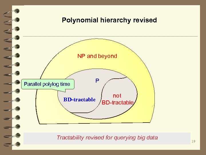
Polynomial hierarchy revised NP and beyond Parallel polylog time BD-tractable P not BD-tractable Tractability revised for querying big data 19
What can we get from BD-tractability? Guidelines for the following. ü What query classes are feasible on big data? ü What query classes can be made feasible to answer on big data? ü How to determine whether it is feasible to answer a class Q of queries on big data? Reduce Q to a complete problem Qc for BDTQ ü If so, how to answer queries in Q? • Compose the reduction and the algorithm for answering queries of Qc Why we need to study theory for querying big data 20
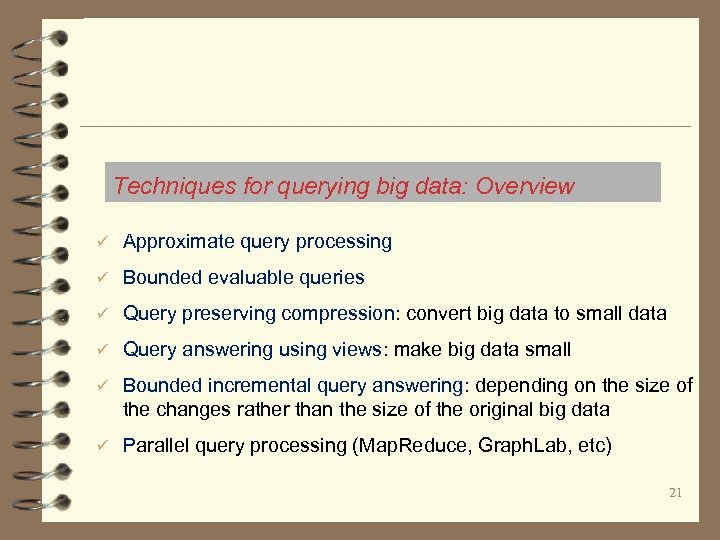
Techniques for querying big data: Overview ü Approximate query processing ü Bounded evaluable queries ü Query preserving compression: convert big data to small data ü Query answering using views: make big data small ü Bounded incremental query answering: depending on the size of the changes rather than the size of the original big data ü Parallel query processing (Map. Reduce, Graph. Lab, etc) 21
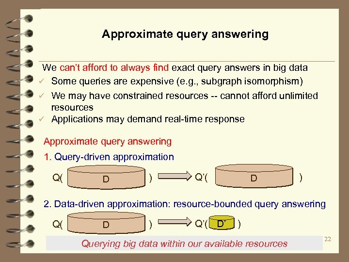
Approximate query answering We can’t afford to always find exact query answers in big data ü Some queries are expensive (e. g. , subgraph isomorphism) ü We may have constrained resources -- cannot afford unlimited resources ü Applications may demand real-time response Approximate query answering 1. Query-driven approximation Q( ) D Q’( ) D 2. Data-driven approximation: resource-bounded query answering Q( ) D Q’( ) D’ Querying big data within our available resources 22
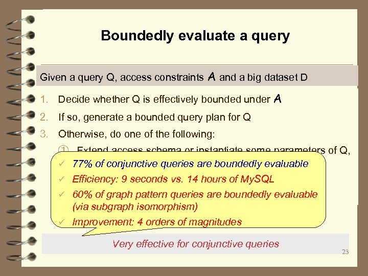
Boundedly evaluate a query Given a query Q, access constraints A and a big dataset D 1. Decide whether Q is effectively bounded under A 2. If so, generate a bounded query plan for Q 3. Otherwise, do one of the following: ① Extend access schema or instantiate some parameters of Q, ü 77% of conjunctive queries are boundedly evaluable to make Q effectively bounded ü Efficiency: 9 seconds vs. 14 hours of My. SQL ② Use other tricks to make D small ü 60% of graph pattern queries are boundedly evaluable ③ Compute approximate query answers to Q in D (via subgraph isomorphism) ü Improvement: 4 orders of magnitudes Very effective for conjunctive queries 23
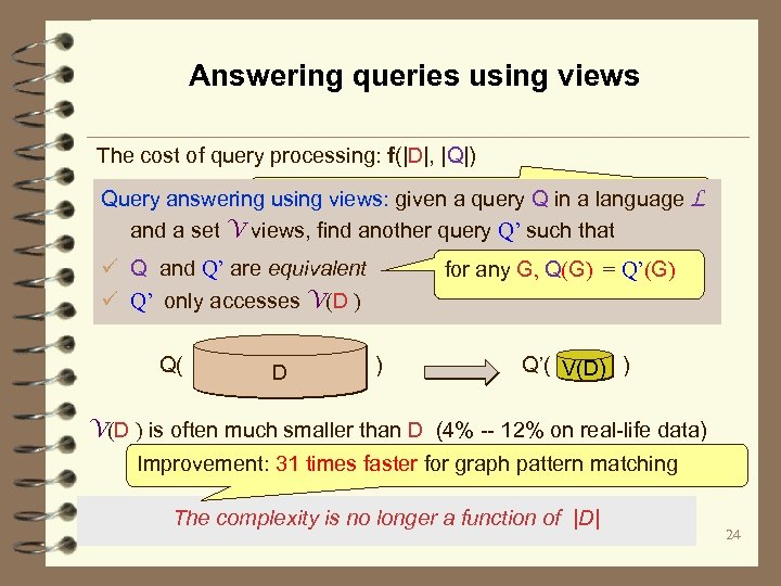
Answering queries using views The cost of query processing: f(|D|, |Q|) can we compute Q(G) without accessing G, i. e. , Query answering using views: given a query Q in a language L independent of |G|? and a set V views, find another query Q’ such that ü Q and Q’ are equivalent ü Q’ only accesses V(D ) Q( ) D for any G, Q(G) = Q’(G) Q’( ) V(D ) is often much smaller than D (4% -- 12% on real-life data) Improvement: 31 times faster for graph pattern matching The complexity is no longer a function of |D| 24
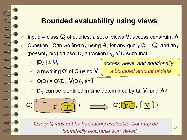
Bounded evaluability using views ü ü Input: A class Q of queries, a set of views V, access constraint A Question: Can we find by using A, for any query Q Q and any (possibly big) dataset D, a fraction DQ of D such that ü |DQ | M, ü Q(D) = Q’(DQ, V(D)), and ü DQ can be identified in time determined by Q, V, and A? access views, and additionally a bounded amount of data ü a rewriting Q’ of Q using V, Q( ) D DQ Q’( , ) V DQ Query Q may not be boundedly evaluable, but may be boundedly evaluable with views! 25
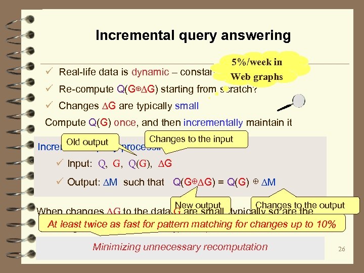
Incremental query answering 5%/week in ü Real-life data is dynamic – constantly changes, ∆G Web graphs ü Re-compute Q(G⊕∆G) starting from scratch? ü Changes ∆G are typically small Compute Q(G) once, and then incrementally maintain it Old output Changes to the input Incremental query processing: ü Input: Q, G, Q(G), ∆G ü Output: ∆M such that Q(G⊕∆G) = Q(G) ⊕ ∆M New output Changes to the output When changes ∆G to the data G are small, typically so are the At least twice to the output Q(G⊕matching for changes up to 10% changes ∆M as fast for pattern ∆G) Minimizing unnecessary recomputation 26
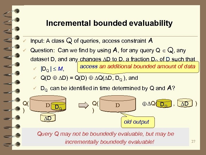
Incremental bounded evaluability ü ü Input: A class Q of queries, access constraint A Question: Can we find by using A, for any query Q Q, any dataset D, and any changes D to D, a fraction DQ of D such that access an additional bounded amount of data ü |D | M, Q ü Q(D D) = Q(D) Q( D, DQ ), and ü DQ can be identified in time determined by Q and A? Q( D D Q ) D Q( , ) D DQ D ) old output Query Q may not be boundedly evaluable, but may be incrementally boundedly evaluable! 27
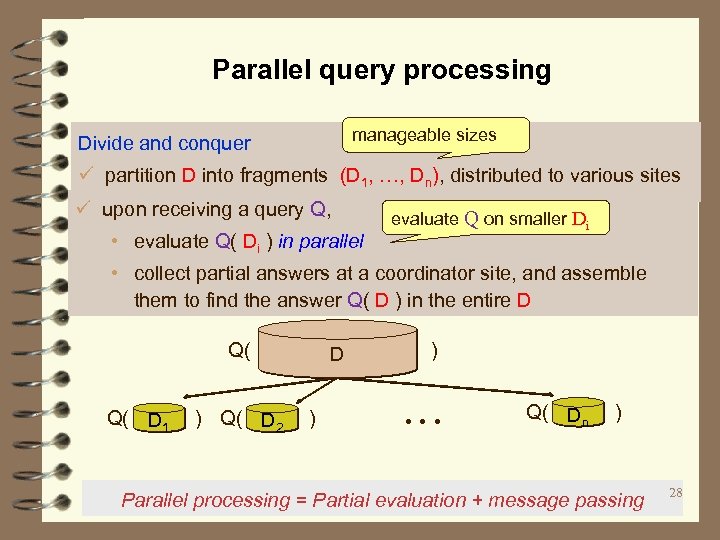
Parallel query processing manageable sizes Divide and conquer ü partition D into fragments (D 1, …, Dn), distributed to various sites ü upon receiving a query Q, • evaluate Q( Di ) in parallel evaluate Q on smaller Di • collect partial answers at a coordinator site, and assemble them to find the answer Q( D ) in the entire D Q( Q( ) D 1 D 2 D ) … Q( ) Dn Parallel processing = Partial evaluation + message passing 28
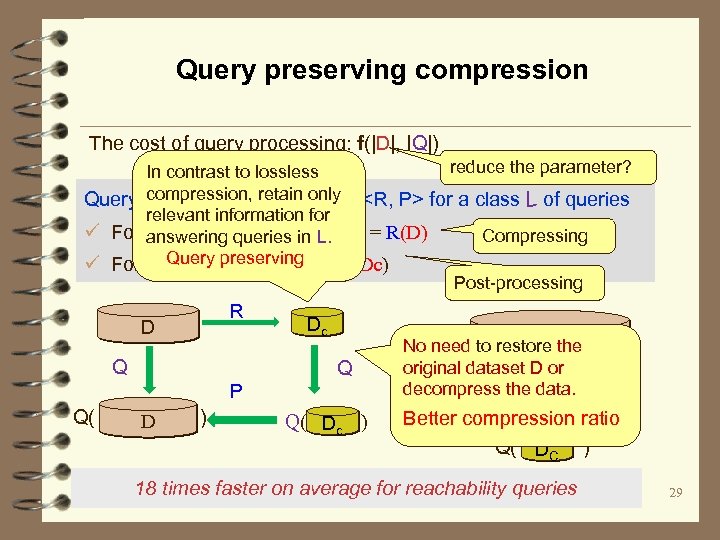
Query preserving compression The cost of query processing: f(|D|, |Q|) reduce the parameter? In contrast to lossless compression, retain only Query preserving compression <R, P> for a class L of queries relevant information for ü For any data collection D, DC = R(D) Compressing answering queries in L. Query preserving ü For any Q in L, Q( D) = P(Q, Dc) Post-processing D R Q Dc Q P Q( ) D Q( Dc ) Q( ) D No need to restore the original dataset D or decompress the data. Better compression ratio Q( ) DC 18 times faster on average for reachability queries 29
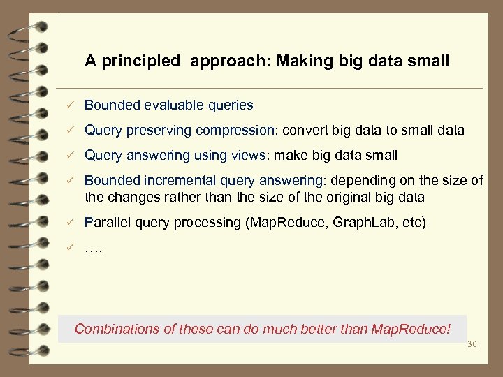
A principled approach: Making big data small ü Bounded evaluable queries ü Query preserving compression: convert big data to small data ü Query answering using views: make big data small ü Bounded incremental query answering: depending on the size of the changes rather than the size of the original big data ü Parallel query processing (Map. Reduce, Graph. Lab, etc) ü …. Combinations of these can do much better than Map. Reduce! 30
Approximate query processing 31
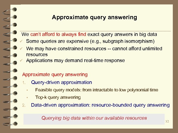
Approximate query answering We can’t afford to always find exact query answers in big data ü Some queries are expensive (e. g. , subgraph isomorphism) ü We may have constrained resources -- cannot afford unlimited resources ü Applications may demand real-time response Approximate query answering Query-driven approximation 1. • • 2. Feasible query models: from intractable to low polynomial time Top-k query answering Data-driven approximation: resource-bounded query answering Querying big data within our available resources 32
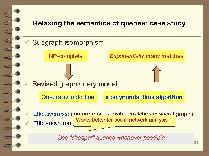
Relaxing the semantics of queries: case study ü Subgraph isomorphism NP-complete ü Exponentially many matches Revised graph query model Quadratic/cubic time a polynomial time algorithm ü Effectiveness: capture more sensible matches in social graphs Works better for social network analysis ü Efficiency: from intractable to low polynomial time Use “cheaper” queries whenever possible 33
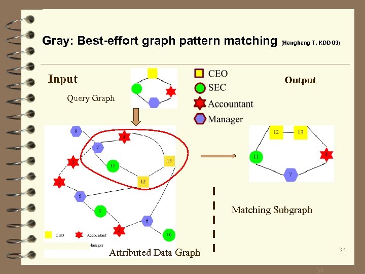
Gray: Best-effort graph pattern matching (Hanghang T. KDD 09) Input Output Query Graph Matching Subgraph 34 Attributed Data Graph 34
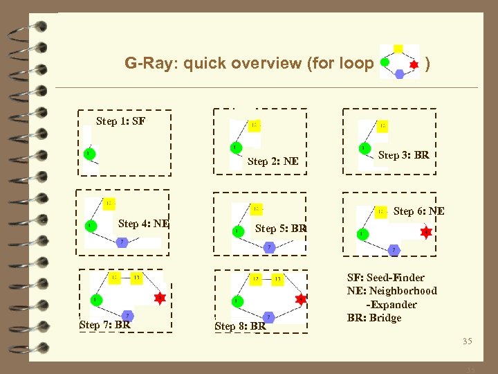
G-Ray: quick overview (for loop ) Step 1: SF Step 2: NE Step 4: NE Step 7: BR Step 3: BR Step 6: NE Step 5: BR Step 8: BR SF: Seed-Finder NE: Neighborhood -Expander BR: Bridge 35 35
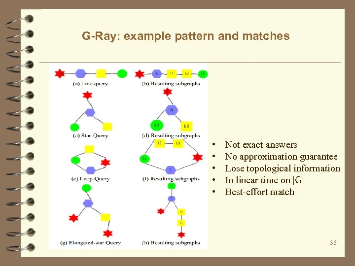
G-Ray: example pattern and matches • • • Not exact answers No approximation guarantee Lose topological information In linear time on |G| Best-effort match 36
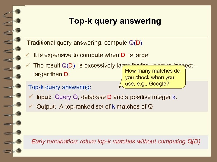
Top-k query answering Traditional query answering: compute Q(D) ü It is expensive to compute when D is large ü The result Q(D) is excessively large for the users to inspect – How many matches do larger than D you check when you use, e. g. , Google? Top-k query answering: ü Input: Query Q, database D and a positive integer k. ü Output: A top-ranked set of k matches of Q Early termination: return top-k matches without computing Q(D) 37
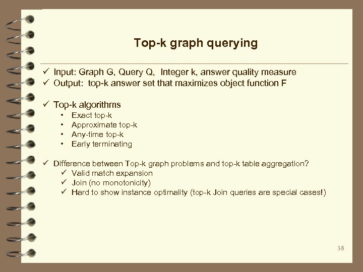
Top-k graph querying ü Input: Graph G, Query Q, Integer k, answer quality measure ü Output: top-k answer set that maximizes object function F ü Top-k algorithms • • Exact top-k Approximate top-k Any-time top-k Early terminating ü Difference between Top-k graph problems and top-k table aggregation? ü Valid match expansion ü Join (no monotonicity) ü Hard to show instance optimality (top-k Join queries are special cases!) 38

Graph. TA: A template Initialize candidate list L for node/edge in Q For each list L nodes/edges of interests sort L with ranking function; Set a cursor to each list; set an upper bound U For each cursor c in each list L do generate a match that contains c; update Q(G, k); update threshold H with lowest score in Q(G, k); move all cursors one step ahead; update the upper bound U; if k matches are identified and H>=U then break; Return Q(G, k) 39
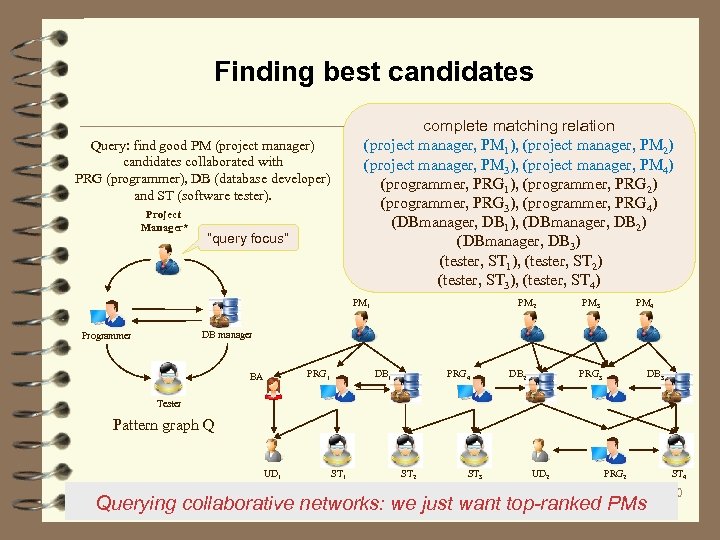
Finding best candidates complete matching relation (project manager, PM 1), (project manager, PM 2) (project manager, PM 3), (project manager, PM 4) (programmer, PRG 1), (programmer, PRG 2) (programmer, PRG 3), (programmer, PRG 4) (DBmanager, DB 1), (DBmanager, DB 2) (DBmanager, DB 3) (tester, ST 1), (tester, ST 2) (tester, ST 3), (tester, ST 4) Query: find good PM (project manager) candidates collaborated with PRG (programmer), DB (database developer) and ST (software tester). Project Manager* “query focus” PM 1 PM 2 PM 3 PM 4 DB manager Programmer BA PRG 1 DB 1 PRG 4 DB 2 PRG 3 DB 3 Tester Pattern graph Q UD 1 ST 2 ST 3 UD 2 PRG 2 Collaboration network G Querying collaborative networks: we just want top-ranked PMs ST 4 40
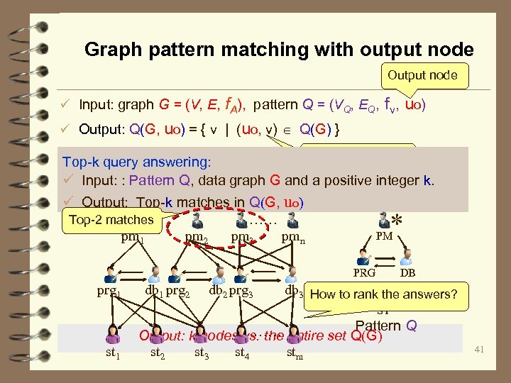
Graph pattern matching with output node Output node ü Input: graph G = (V, E, f. A), pattern Q = (VQ, EQ, fv, uo) ü Output: Q(G, uo) = { v | (uo, v) Q(G) } Matches of the Top-k query answering: output node ü Input: : Pattern Q, data graph G and a positive integer k. ü Output: Top-k matches in Q(G, uo) Top-2 matches …… pm 3 pmn pm 1 pm 2 * PM PRG prg 1 db 1 prg 2 db 2 prg 3 DB db 3 How to rank the answers? ST st 1 Pattern Q …… entire set Q(G) Output: k nodes vs. the st 2 st 3 st 4 stm 41
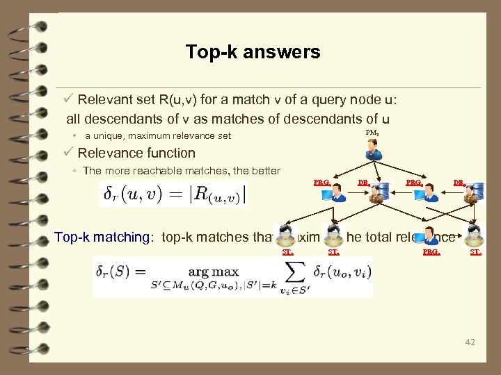
Top-k answers ü Relevant set R(u, v) for a match v of a query node u: all descendants of v as matches of descendants of u PM 2 • a unique, maximum relevance set ü Relevance function ◦ The more reachable matches, the better PRG 4 DB 2 PRG 3 DB 3 Top-k matching: top-k matches that maximize the total relevance ST 2 ST 3 PRG 2 ST 4 42
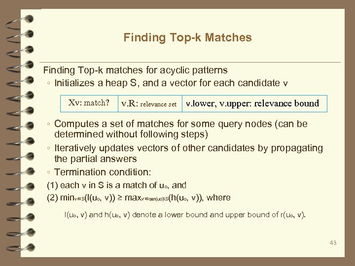
Finding Top-k Matches Finding Top-k matches for acyclic patterns ◦ Initializes a heap S, and a vector for each candidate v x. Xv: match? v. R: relevance set v. lower, v. upper: relevance bound ◦ Computes a set of matches for some query nodes (can be determined without following steps) ◦ Iteratively updates vectors of other candidates by propagating the partial answers ◦ Termination condition: (1) each v in S is a match of uo, and (2) minv∈S(l(uo, v)) ≥ maxv′∈can(uo)S(h(uo, v)), where l(uo, v) and h(uo, v) denote a lower bound and upper bound of r(uo, v). 43
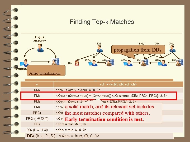
Finding Top-k Matches Project Manager* PM 1 PM 2 PM 3 PM 4 propagation from DB 2 BA PRG 1 DB 1 PRG 4 DB 2 PRG 3 DB manager Programmer After initialization v v v. T = <v. bf, v. R, v. l, v. h> v. T = <v. bf, v. R, v. l, PM PM 1 1 <X<XPM 1 PRG 1 ˄ XDB 1, Ф, 0, 2> PM 1 = XPRG 1 ˄ XDB 1, Ф, 0, 2> PM 2 2 PM <X<XPM 2 = (X =true) V (XPRG 4=true)) ˄ XDB 2=true, {DB 2, PRG 4, PRG 3}, 3, 3> PM 2 = ((XPRG 3 V XPRG 4) ˄ XDB 2, Ф, 0, 3> PM 3 <XPM 3 = (XPRG 3 = true) ˄ (XDB 2=true), {DB 2, PRG 3}, 2, 2> PM 4 <XPM 4 = (XPRG 3 = true) ˄ XDB 3, Ф, 0, 2> a valid match, and its relevant set includes PM 3 PM 4 PRG 1 PRGj (j ∈ [3, 4]) DB 2 PRGj (j ∈ [3, 4]) DBk (k ∈ [1, 3]) <XPM 3 = XPRG 3 ˄ XDB 2, Ф, 0, 2> <XPM 4 = XPRG 3 ˄ XDB 3, Ф, 0, 2> the most matches compared with others. <X<XPRG 1 = XDB 1, Ф, 0, 1> condition is met. = true, {DB 2}, 1, 1> Early termination <XPRG 1 = XDB 1, Ф, 0, 1> PRGj <X<X = true, Ф, 0, 0> DB 2 PRGj = XDB 2, Ф, 0, 1> <XDBk = true, Ф, 0, 0> DBk (k ∈ [1, 3]) <XDBk = true, Ф, 0, 0> DB 3
Reading 1. M. Arenas, L. E. Bertossi, J. Chomicki: Consistent Query Answers in Inconsistent Databases, PODS 1999. http: //web. ing. puc. cl/~marenas/publications/pods 99. pdf 2. Indrajit Bhattacharya and Lise Getoor. Collective Entity Resolution in Relational Data. TKDD, 2007. http: //linqs. cs. umd. edu/basilic/web/Publications/2007/bhattacharya: tkdd 07/bhattac harya-tkdd. pdf 3. P. Li, X. Dong, A. Maurino, and D. Srivastava. Linking Temporal Records. VLDB 2011. http: //www. vldb. org/pvldb/vol 4/p 956 -li. pdf 4. W. Fan and F. Geerts,Relative information completeness, PODS, 2009. 5. Y. Cao. W. Fan, and W. Yu. Determining relative accuracy of attributes. SIGMOD 2013. 6. P. Buneman, S. Davidson, W. Fan, C. Hara and W. Tan. Keys for XML. WWW 2001. 45
9ec3f5ac9e4841b83d44a52f08cecdf7.ppt