0d7d7b01b8b30b67698a410f610437d9.ppt
- Количество слайдов: 53
CPT-S 415 Topics in Computer Science Big Data Yinghui Wu EME B 45 1
CPT-S 415 Big Data Special topic: Data Mining & Graph Mining ü Data mining: from data to knowledge ü Graph Mining ü Classification (next week) ü Clustering (next week) 2
Data Mining Basics 3
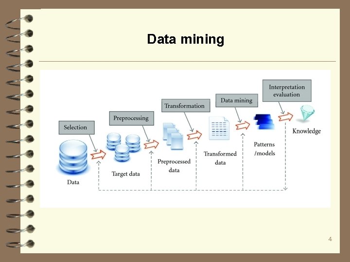
Data mining ü What is data mining? A tentative definition: – Use of efficient techniques for analysis of very large collections of data and the extraction of useful and possibly unexpected patterns in data – Non-trivial extraction of implicit, previously unknown and potentially useful information from data – Exploration & analysis, by automatic or semi-automatic means, of large quantities of data in order to discover meaningful patterns Data 4
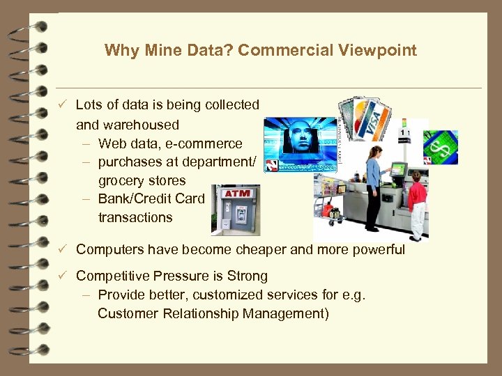
Why Mine Data? Commercial Viewpoint ü Lots of data is being collected and warehoused – Web data, e-commerce – purchases at department/ grocery stores – Bank/Credit Card transactions ü Computers have become cheaper and more powerful ü Competitive Pressure is Strong – Provide better, customized services for e. g. Customer Relationship Management)
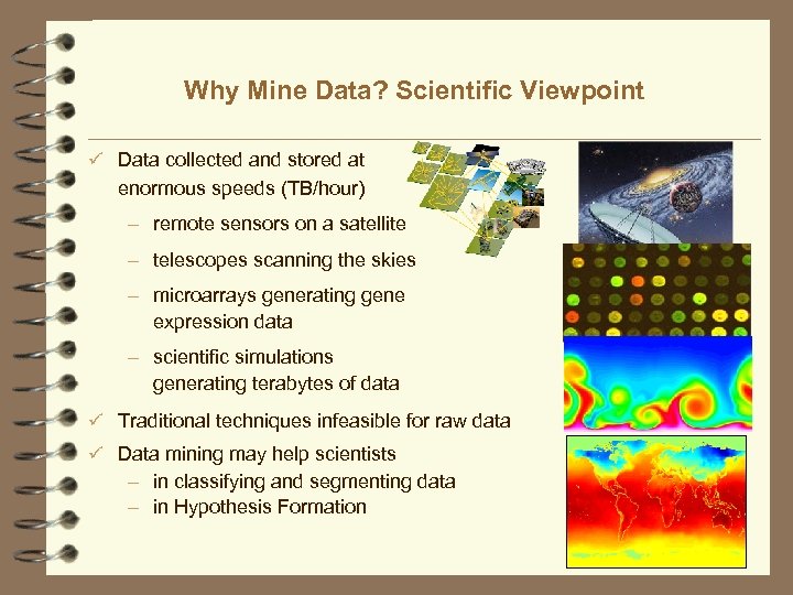
Why Mine Data? Scientific Viewpoint ü Data collected and stored at enormous speeds (TB/hour) – remote sensors on a satellite – telescopes scanning the skies – microarrays generating gene expression data – scientific simulations generating terabytes of data ü Traditional techniques infeasible for raw data ü Data mining may help scientists – in classifying and segmenting data – in Hypothesis Formation
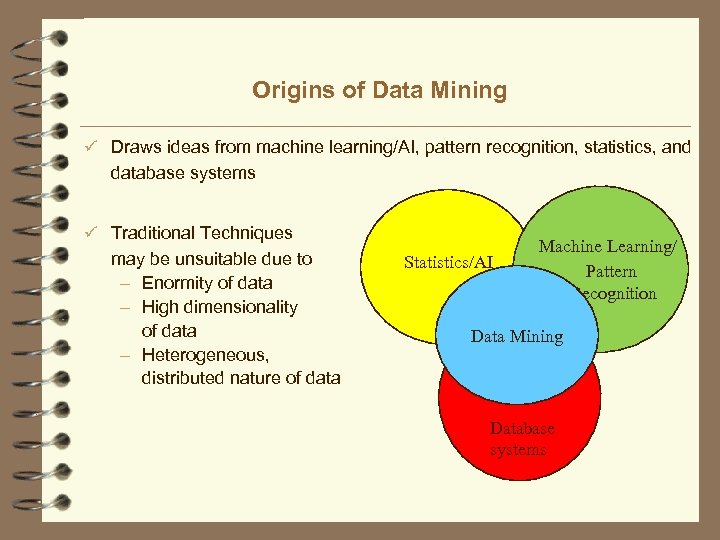
Origins of Data Mining ü Draws ideas from machine learning/AI, pattern recognition, statistics, and database systems ü Traditional Techniques may be unsuitable due to – Enormity of data – High dimensionality of data – Heterogeneous, distributed nature of data Statistics/AI Machine Learning/ Pattern Recognition Data Mining Database systems
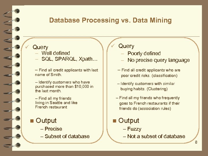
Database Processing vs. Data Mining ü Query – Well defined – SQL, SPARQL, Xpath… ü Query – Poorly defined – No precise query language – Find all credit applicants with last – Find all credit applicants who are name of Smith. poor credit risks. (classification) – Identify customers who have purchased more than $10, 000 in the last month. – Find all my friends living in Seattle and like French restaurant n – Identify customers with similar buying habits. (Clustering) – Find all my friends who frequently goes to French restaurants if their friends do (association rules) Output – Precise – Subset of database n Output – Fuzzy – Not a subset of database 8
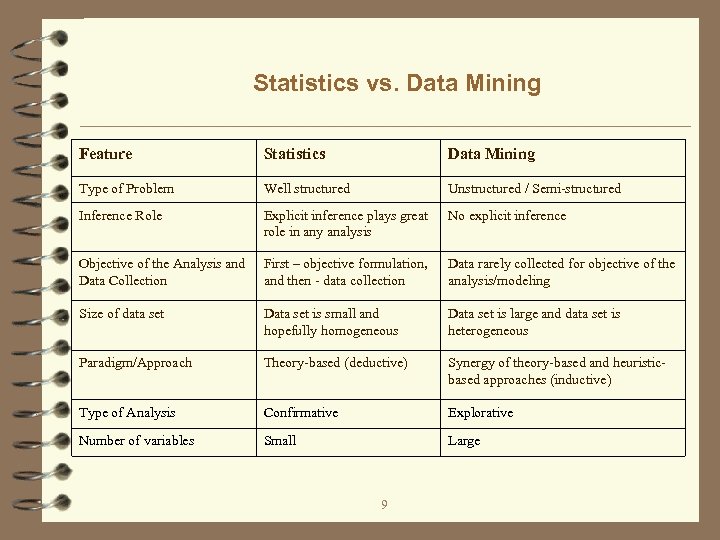
Statistics vs. Data Mining Feature Statistics Data Mining Type of Problem Well structured Unstructured / Semi-structured Inference Role Explicit inference plays great role in any analysis No explicit inference Objective of the Analysis and Data Collection First – objective formulation, and then - data collection Data rarely collected for objective of the analysis/modeling Size of data set Data set is small and hopefully homogeneous Data set is large and data set is heterogeneous Paradigm/Approach Theory-based (deductive) Synergy of theory-based and heuristicbased approaches (inductive) Type of Analysis Confirmative Explorative Number of variables Small Large 9
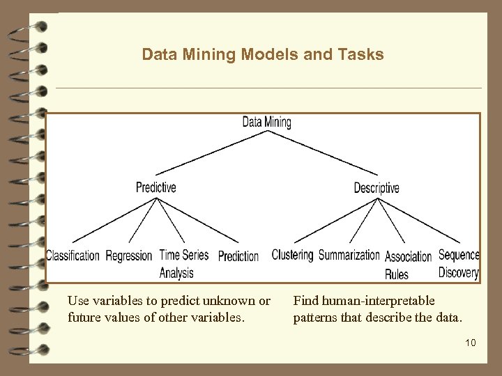
Data Mining Models and Tasks Use variables to predict unknown or future values of other variables. Find human-interpretable patterns that describe the data. 10
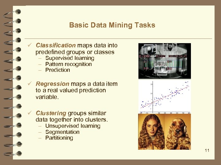
Basic Data Mining Tasks ü Classification maps data into predefined groups or classes – Supervised learning – Pattern recognition – Prediction ü Regression maps a data item to a real valued prediction variable. ü Clustering groups similar data together into clusters. – Unsupervised learning – Segmentation – Partitioning 11
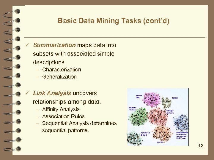
Basic Data Mining Tasks (cont’d) ü Summarization maps data into subsets with associated simple descriptions. – Characterization – Generalization ü Link Analysis uncovers relationships among data. – Affinity Analysis – Association Rules – Sequential Analysis determines sequential patterns. 12
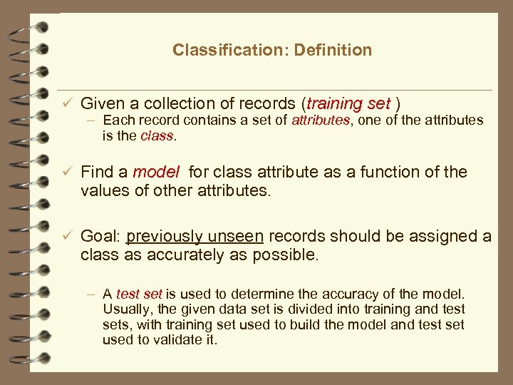
Classification: Definition ü Given a collection of records (training set ) – Each record contains a set of attributes, one of the attributes is the class. ü Find a model for class attribute as a function of the values of other attributes. ü Goal: previously unseen records should be assigned a class as accurately as possible. – A test set is used to determine the accuracy of the model. Usually, the given data set is divided into training and test sets, with training set used to build the model and test set used to validate it.
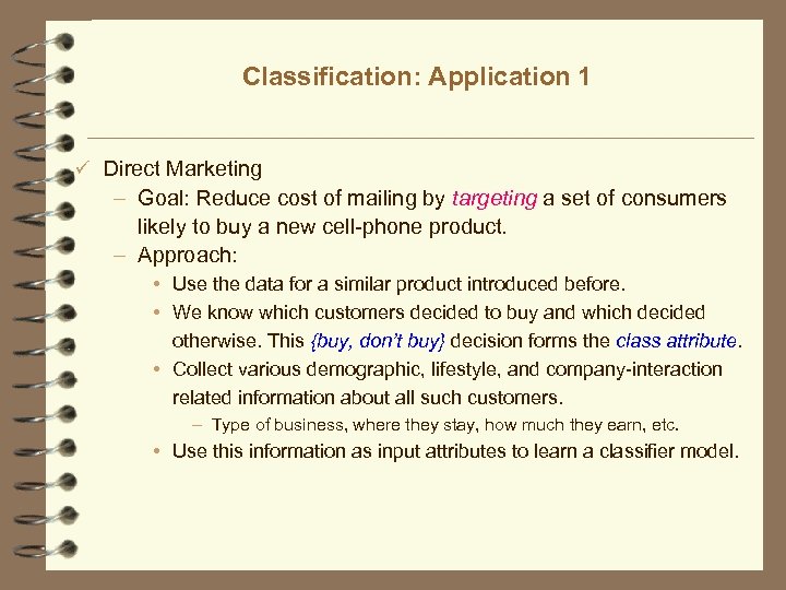
Classification: Application 1 ü Direct Marketing – Goal: Reduce cost of mailing by targeting a set of consumers likely to buy a new cell-phone product. – Approach: • Use the data for a similar product introduced before. • We know which customers decided to buy and which decided otherwise. This {buy, don’t buy} decision forms the class attribute. • Collect various demographic, lifestyle, and company-interaction related information about all such customers. – Type of business, where they stay, how much they earn, etc. • Use this information as input attributes to learn a classifier model.
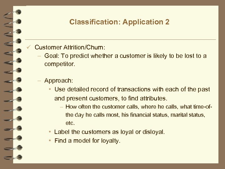
Classification: Application 2 ü Customer Attrition/Churn: – Goal: To predict whether a customer is likely to be lost to a competitor. – Approach: • Use detailed record of transactions with each of the past and present customers, to find attributes. – How often the customer calls, where he calls, what time-ofthe day he calls most, his financial status, marital status, etc. • Label the customers as loyal or disloyal. • Find a model for loyalty.
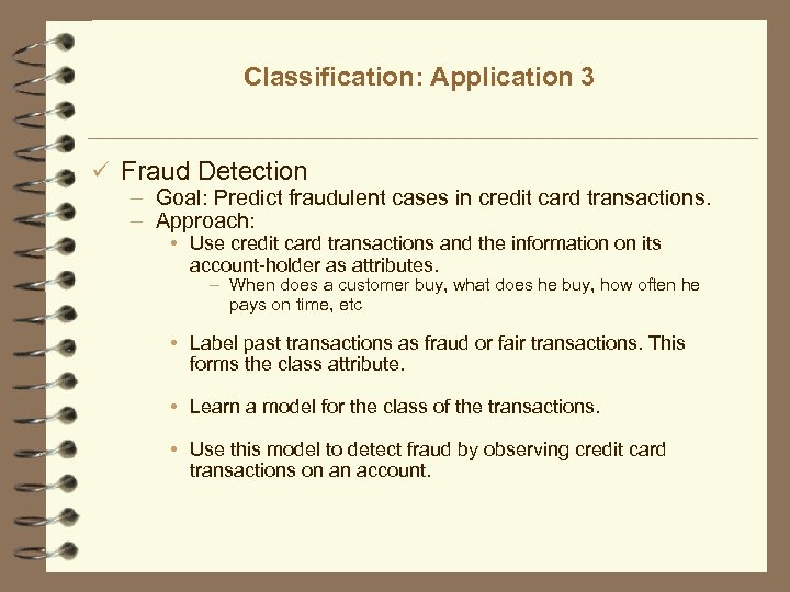
Classification: Application 3 ü Fraud Detection – Goal: Predict fraudulent cases in credit card transactions. – Approach: • Use credit card transactions and the information on its account-holder as attributes. – When does a customer buy, what does he buy, how often he pays on time, etc • Label past transactions as fraud or fair transactions. This forms the class attribute. • Learn a model for the class of the transactions. • Use this model to detect fraud by observing credit card transactions on an account.
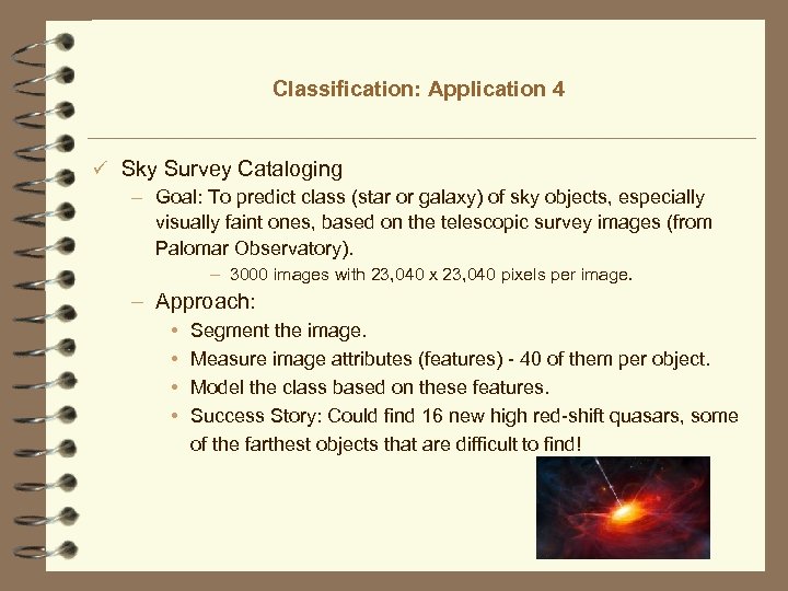
Classification: Application 4 ü Sky Survey Cataloging – Goal: To predict class (star or galaxy) of sky objects, especially visually faint ones, based on the telescopic survey images (from Palomar Observatory). – 3000 images with 23, 040 x 23, 040 pixels per image. – Approach: • • Segment the image. Measure image attributes (features) - 40 of them per object. Model the class based on these features. Success Story: Could find 16 new high red-shift quasars, some of the farthest objects that are difficult to find!
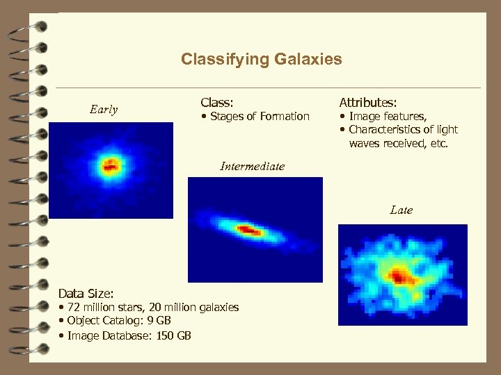
Classifying Galaxies Early Class: • Stages of Formation Attributes: • Image features, • Characteristics of light waves received, etc. Intermediate Late Data Size: • 72 million stars, 20 million galaxies • Object Catalog: 9 GB • Image Database: 150 GB
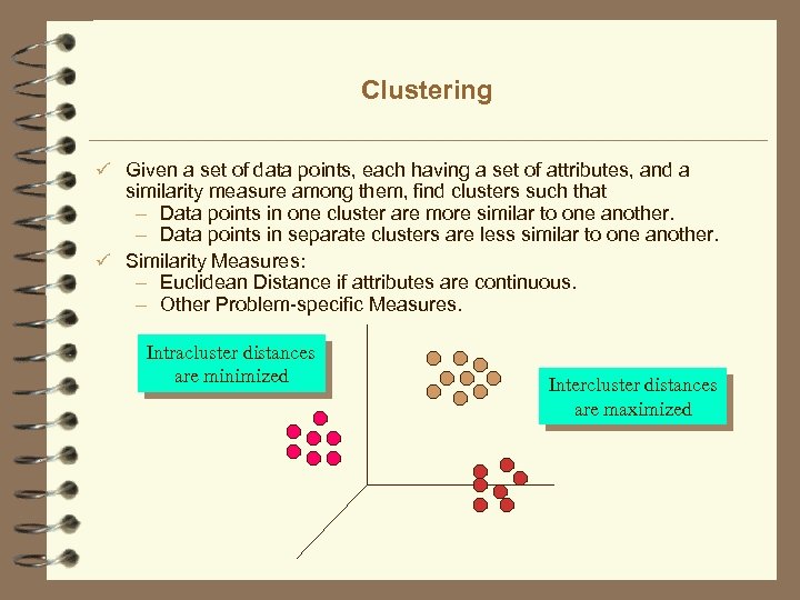
Clustering ü Given a set of data points, each having a set of attributes, and a similarity measure among them, find clusters such that – Data points in one cluster are more similar to one another. – Data points in separate clusters are less similar to one another. ü Similarity Measures: – Euclidean Distance if attributes are continuous. – Other Problem-specific Measures. Intracluster distances are minimized Intercluster distances are maximized
Clustering: Application 1 ü Market Segmentation: – Goal: subdivide a market into distinct subsets of customers where any subset may conceivably be selected as a market target to be reached with a distinct marketing mix. – Approach: • Collect different attributes of customers based on their geographical and lifestyle related information. • Find clusters of similar customers. • Measure the clustering quality by observing buying patterns of customers in same cluster vs. those from different clusters.
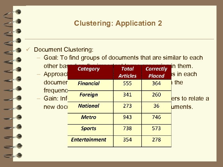
Clustering: Application 2 ü Document Clustering: – Goal: To find groups of documents that are similar to each other based on the important terms appearing in them. – Approach: To identify frequently occurring terms in each document. Form a similarity measure based on the frequencies of different terms. Use it to cluster. – Gain: Information Retrieval can utilize the clusters to relate a new document or search term to clustered documents.
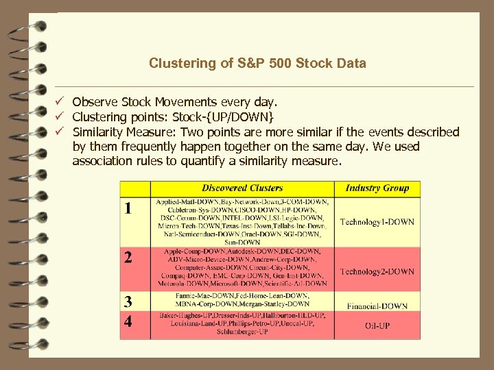
Clustering of S&P 500 Stock Data ü Observe Stock Movements every day. ü Clustering points: Stock-{UP/DOWN} ü Similarity Measure: Two points are more similar if the events described by them frequently happen together on the same day. We used association rules to quantify a similarity measure.
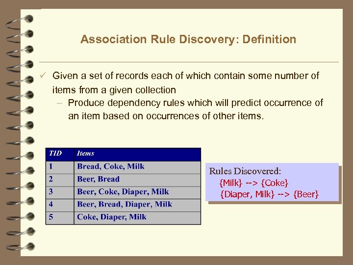
Association Rule Discovery: Definition ü Given a set of records each of which contain some number of items from a given collection – Produce dependency rules which will predict occurrence of an item based on occurrences of other items. Rules Discovered: {Milk} --> {Coke} {Diaper, Milk} --> {Beer}
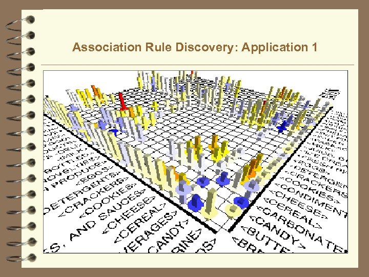
Association Rule Discovery: Application 1 ü Marketing and Sales Promotion: – Let the rule discovered be {Bagels, … } --> {Potato Chips} – Potato Chips as consequent => Can be used to determine what should be done to boost its sales. – Bagels in the antecedent => Can be used to see which products would be affected if the store discontinues selling bagels. – Bagels in antecedent and Potato chips in consequent => Can be used to see what products should be sold with Bagels to promote sale of Potato chips
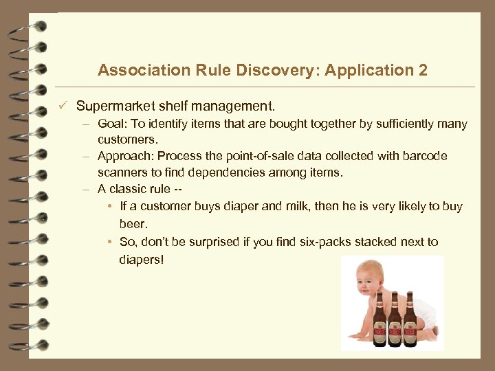
Association Rule Discovery: Application 2 ü Supermarket shelf management. – Goal: To identify items that are bought together by sufficiently many customers. – Approach: Process the point-of-sale data collected with barcode scanners to find dependencies among items. – A classic rule - • If a customer buys diaper and milk, then he is very likely to buy beer. • So, don’t be surprised if you find six-packs stacked next to diapers!
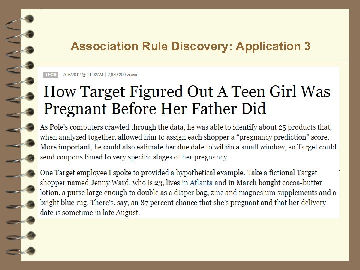
Association Rule Discovery: Application 3 ü Inventory Management – Goal: A consumer appliance repair company wants to anticipate the nature of repairs on its consumer products and keep the service vehicles equipped with right parts to reduce on number of visits to consumer households. – Approach: Process the data on tools and parts required in previous repairs at different consumer locations and discover the co-occurrence patterns.
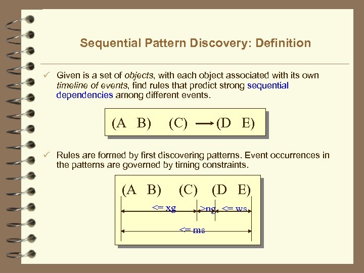
Sequential Pattern Discovery: Definition ü Given is a set of objects, with each object associated with its own timeline of events, find rules that predict strong sequential dependencies among different events. (A B) (C) (D E) ü Rules are formed by first discovering patterns. Event occurrences in the patterns are governed by timing constraints. (A B) <= xg (C) (D E) >ng <= ws <= ms
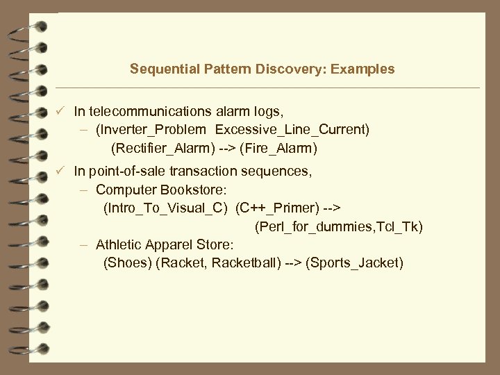
Sequential Pattern Discovery: Examples ü In telecommunications alarm logs, – (Inverter_Problem Excessive_Line_Current) (Rectifier_Alarm) --> (Fire_Alarm) ü In point-of-sale transaction sequences, – Computer Bookstore: (Intro_To_Visual_C) (C++_Primer) --> (Perl_for_dummies, Tcl_Tk) – Athletic Apparel Store: (Shoes) (Racket, Racketball) --> (Sports_Jacket)
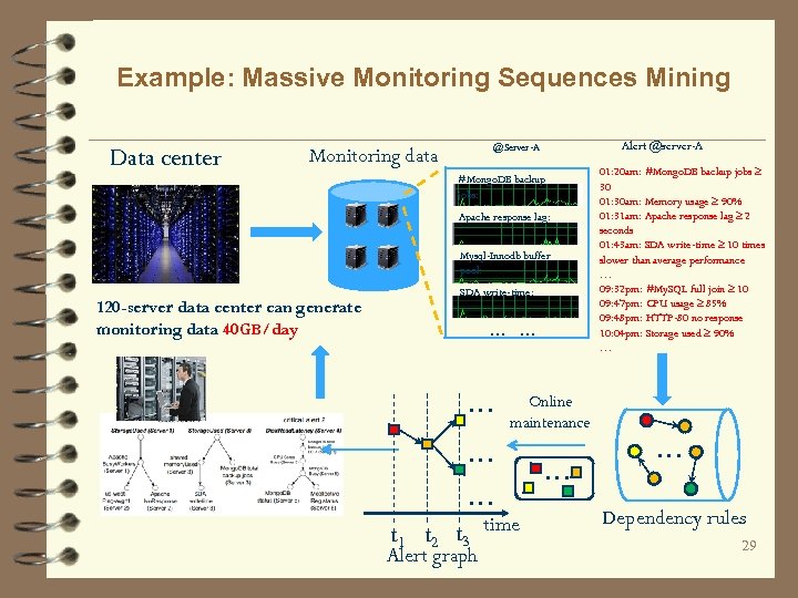
Example: Massive Monitoring Sequences Mining Data center Monitoring data Alert @server-A @Server-A #Mongo. DB backup jobs: Apache response lag: Mysql-Innodb buffer pool: 120 -server data center can generate monitoring data 40 GB/day SDA write-time: … … … 01: 20 am: #Mongo. DB backup jobs ≥ 30 01: 30 am: Memory usage ≥ 90% 01: 31 am: Apache response lag ≥ 2 seconds 01: 43 am: SDA write-time ≥ 10 times slower than average performance … 09: 32 pm: #My. SQL full join ≥ 10 09: 47 pm: CPU usage ≥ 85% 09: 48 pm: HTTP-80 no response 10: 04 pm: Storage used ≥ 90% … Online maintenance … … time t 1 t 2 t 3 Alert graph … … Dependency rules 29
Regression ü Predict a value of a given continuous valued variable based on the values of other variables, assuming a linear or nonlinear model of dependency. ü Greatly studied in statistics, neural network fields. ü Examples: – Predicting sales amounts of new product based on advertising expenditure. – Predicting wind velocities as a function of temperature, humidity, air pressure, etc. – Time series prediction of stock market indices.
Challenges of Data Mining ü Scalability ü Dimensionality ü Complex and Heterogeneous Data ü Data Quality ü Data Ownership and Distribution ü Privacy Preservation ü Streaming Data
Graph Mining 32
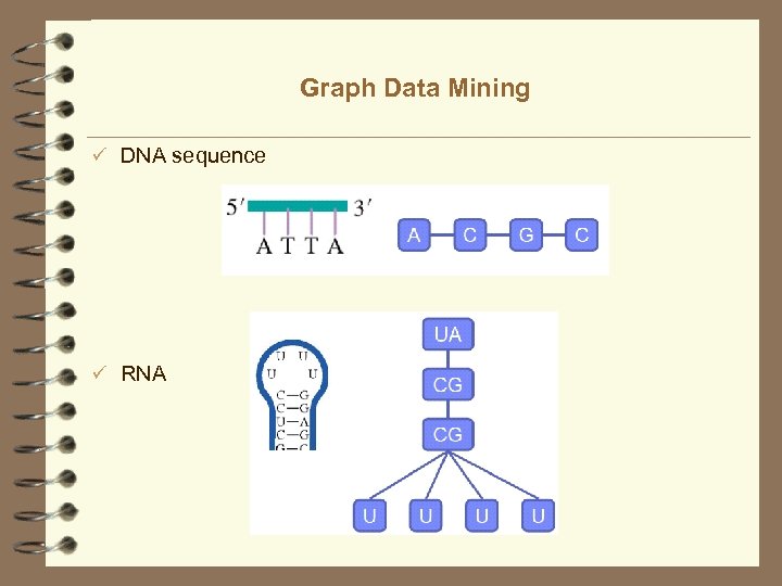
Graph Data Mining ü DNA sequence ü RNA
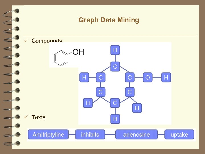
Graph Data Mining ü Compounds ü Texts
Graph Mining ü Graph Pattern Mining – Mining Frequent Subgraph Patterns – Graph Indexing – Graph Similarity Search ü Graph Classification – Graph pattern-based approach – Machine Learning approaches ü Graph Clustering – Link-density-based approach
Graph Pattern Mining 36
Graph Pattern Mining ü Frequent subgraphs – A (sub)graph is frequent if its support (occurrence frequency) in a given dataset is no less than a minimum support threshold ü Support of a graph g is defined as the percentage of graphs in G which have g as subgraph ü Applications of graph pattern mining – Mining biochemical structures – Program control flow analysis – Mining XML structures or Web communities – Building blocks for graph classification, clustering, compression, comparison, and correlation analysis 36
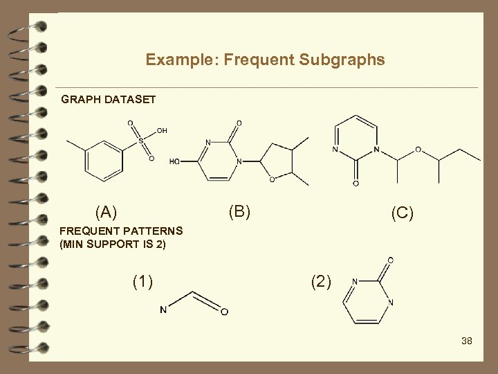
Example: Frequent Subgraphs GRAPH DATASET (B) (A) (C) FREQUENT PATTERNS (MIN SUPPORT IS 2) (1) (2) 38
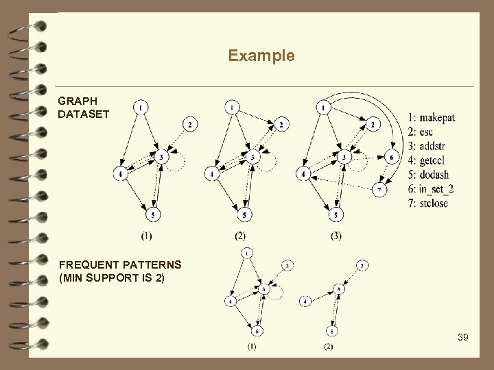
Example GRAPH DATASET FREQUENT PATTERNS (MIN SUPPORT IS 2) 39
Graph Mining Algorithms ü Incomplete beam search – Greedy (Subdue) ü Inductive logic programming (WARMR) ü Graph theory-based approaches – Apriori-based approach – Pattern-growth approach 40
Properties of Graph Mining Algorithms ü Search order – breadth vs. depth ü Generation of candidate subgraphs – apriori vs. pattern growth ü Elimination of duplicate subgraphs – passive vs. active ü Support calculation – embedding store or not ü Discover order of patterns – path tree graph 41
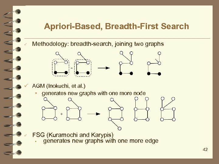
Apriori-Based, Breadth-First Search ü Methodology: breadth-search, joining two graphs ü AGM (Inokuchi, et al. ) • generates new graphs with one more node ü FSG (Kuramochi and Karypis) • generates new graphs with one more edge 42
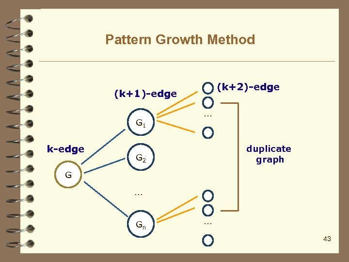
Pattern Growth Method (k+2)-edge (k+1)-edge G 1 k-edge … duplicate graph G 2 G … Gn … 43
Graph Pattern Explosion Problem ü If a graph is frequent, all of its subgraphs are frequent – the Apriori property ü An n-edge frequent graph may have 2 n subgraphs ü Among 422 chemical compounds which are confirmed to be active in an AIDS antiviral screen dataset, – there are 1, 000 frequent graph patterns if the minimum support is 5% 44
Closed Frequent Graphs ü A frequent graph G is closed – if there exists no supergraph of G that carries the same support as G ü If some of G’s subgraphs have the same support – it is unnecessary to output these subgraphs – nonclosed graphs ü Lossless compression – Still ensures that the mining result is complete
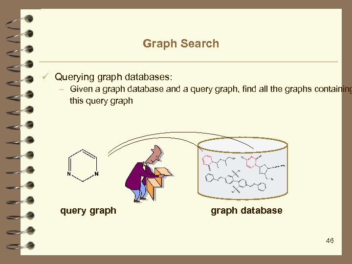
Graph Search ü Querying graph databases: – Given a graph database and a query graph, find all the graphs containing this query graph database 46
Scalability Issue ü Naïve solution – Sequential scan (Disk I/O) – Subgraph isomorphism test (NP-complete) ü Problem: Scalability is a big issue ü An indexing mechanism is needed 47
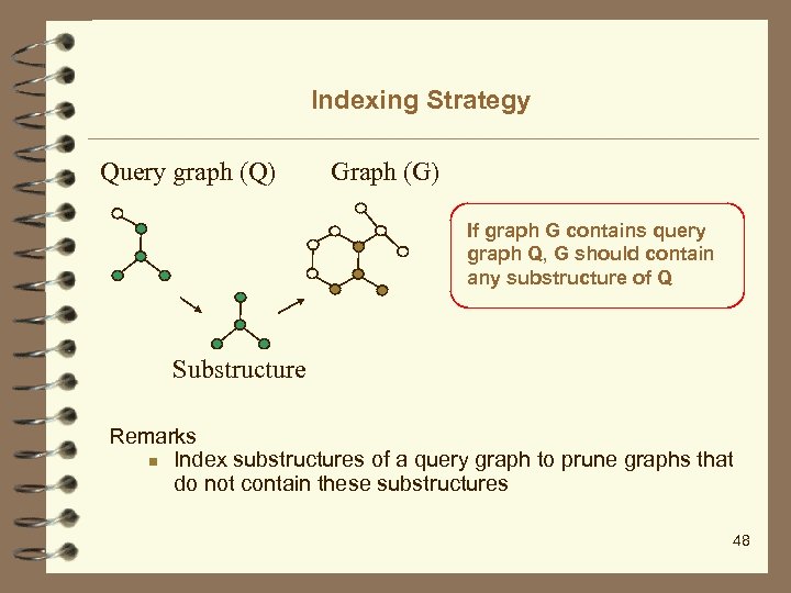
Indexing Strategy Query graph (Q) Graph (G) If graph G contains query graph Q, G should contain any substructure of Q Substructure Remarks n Index substructures of a query graph to prune graphs that do not contain these substructures 48
Indexing Framework ü Two steps in processing graph queries Step 1. Index Construction n Enumerate structures in the graph database, build an inverted index between structures and graphs Step 2. Query Processing n Enumerate structures in the query graph n Calculate the candidate graphs containing these structures n Prune the false positive answers by performing subgraph isomorphism test 49
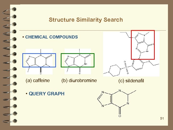
Structure Similarity Search • CHEMICAL COMPOUNDS (a) caffeine (b) diurobromine (c) sildenafil • QUERY GRAPH 51
Substructure Similarity Measure ü Feature-based similarity measure – Each graph is represented as a feature vector X = {x 1, x 2, …, xn} – Similarity is defined by the distance of their corresponding vectors – Advantages • Easy to index • Fast • Rough measure 52
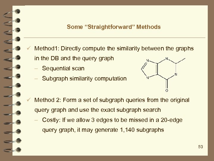
Some “Straightforward” Methods ü Method 1: Directly compute the similarity between the graphs in the DB and the query graph – Sequential scan – Subgraph similarity computation ü Method 2: Form a set of subgraph queries from the original query graph and use the exact subgraph search – Costly: If we allow 3 edges to be missed in a 20 -edge query graph, it may generate 1, 140 subgraphs 53
Index: Precise vs. Approximate Search ü Precise Search – Use frequent patterns as indexing features – Select features in the database space based on their selectivity – Build the index ü Approximate Search – Hard to build indices covering similar subgraphs • explosive number of subgraphs in databases – Idea: (1) keep the index structure (2) select features in the query space 54
0d7d7b01b8b30b67698a410f610437d9.ppt