COURSE SYLLABUS Course Title Managerial Economics Credit

COURSE SYLLABUS Course Title : Managerial Economics Credit Hours : 3 Hours Prerequisites : Microeconomics Professor Name : Dr. Fakhry El-Fiky Email Address : [email protected] com Text Book : Paul G. Keat, And Philip K. Y. Young, Managerial Economics : Economic Tools for Today’s Decision Makers, Fifth Edition. Pearson Education International, 2006. 1

COURSE OBJECTIVES The aim of this course is to present a clear understanding of the principles of managerial decision-making. which lays the foundation for a comprehensive awareness of what is going on a round us in the real business world. To that end, the professor together with the participants will review the basic microeconomic concepts and theories that are centered toward the consumer and firm economic rational behavior. 2

TEACHING TOOLS Lecture : Coverage of course material using power point slides Home & Class Assignments: Four assignments. A gradual development of the graduate student’s interactive learning skills and Invest more time in deepening the participants understanding of the course material. Case Studies : Each chapter opens with a real-life mini-case studies, that is developed through the chapter. Examples from all over The world , and the following mini-case studies are demonstrated and discussed in depth. Exams : mid-term, and a final exams. 3

COURSE EVALUATION & REQUIREMENTS Evaluation System Participation & Assignments : Midterm Exam : Final Exam : Weight 20 % 60 % Requirements Attendance : Participants are advised to attend classes in timely fashion. Attendance is an important element in the evaluation system. Make up Policy : All assignments should be handed in on timely manner. Make ups for some missing academic works may be granted in exceptional circumstances. Format of assignments: All assignment and take-home exams are to Be typed , not hand written 4

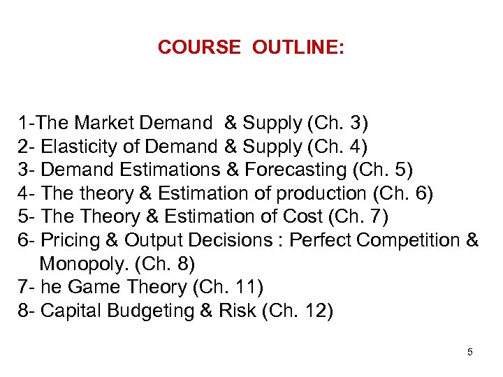
COURSE OUTLINE: 1 -The Market Demand & Supply (Ch. 3) 2 - Elasticity of Demand & Supply (Ch. 4) 3 - Demand Estimations & Forecasting (Ch. 5) 4 - The theory & Estimation of production (Ch. 6) 5 - Theory & Estimation of Cost (Ch. 7) 6 - Pricing & Output Decisions : Perfect Competition & Monopoly. (Ch. 8) 7 - he Game Theory (Ch. 11) 8 - Capital Budgeting & Risk (Ch. 12) 5

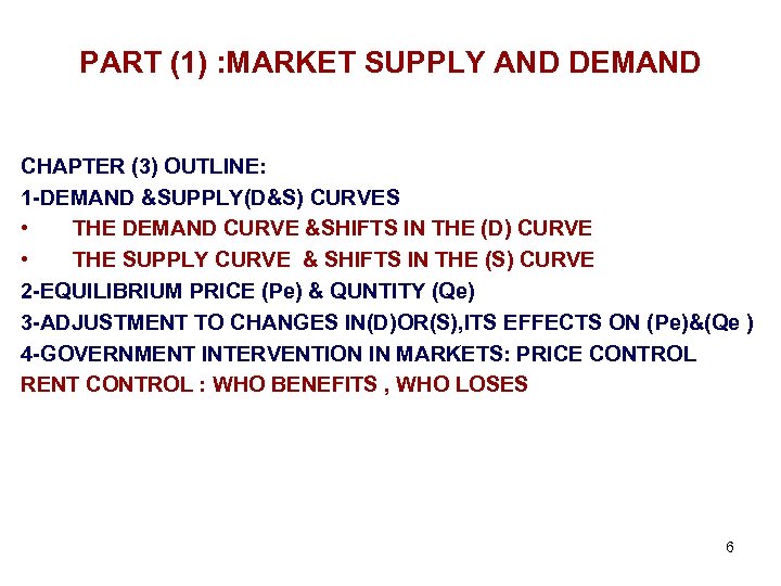
PART (1) : MARKET SUPPLY AND DEMAND CHAPTER (3) OUTLINE: 1 -DEMAND &SUPPLY(D&S) CURVES • THE DEMAND CURVE &SHIFTS IN THE (D) CURVE • THE SUPPLY CURVE & SHIFTS IN THE (S) CURVE 2 -EQUILIBRIUM PRICE (Pe) & QUNTITY (Qe) 3 -ADJUSTMENT TO CHANGES IN(D)OR(S), ITS EFFECTS ON (Pe)&(Qe ) 4 -GOVERNMENT INTERVENTION IN MARKETS: PRICE CONTROL RENT CONTROL : WHO BENEFITS , WHO LOSES 6

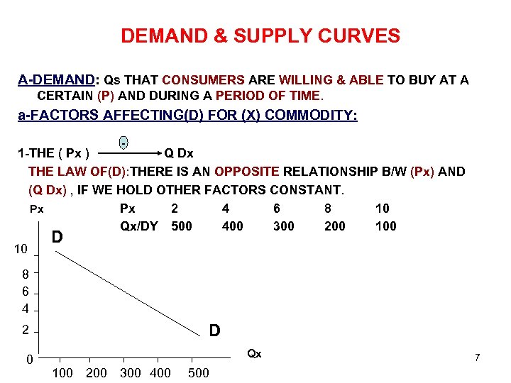
DEMAND & SUPPLY CURVES A-DEMAND: Qs THAT CONSUMERS ARE WILLING & ABLE TO BUY AT A CERTAIN (P) AND DURING A PERIOD OF TIME. a-FACTORS AFFECTING(D) FOR (X) COMMODITY: - 1 -THE ( Px ) Q Dx THE LAW OF(D): THERE IS AN OPPOSITE RELATIONSHIP B/W (Px) AND (Q Dx) , IF WE HOLD OTHER FACTORS CONSTANT. Px 2 4 6 8 10 Px Qx/DY 500 400 300 200 10 D 8 6 4 D 2 0 Qx 100 200 300 400 500 7

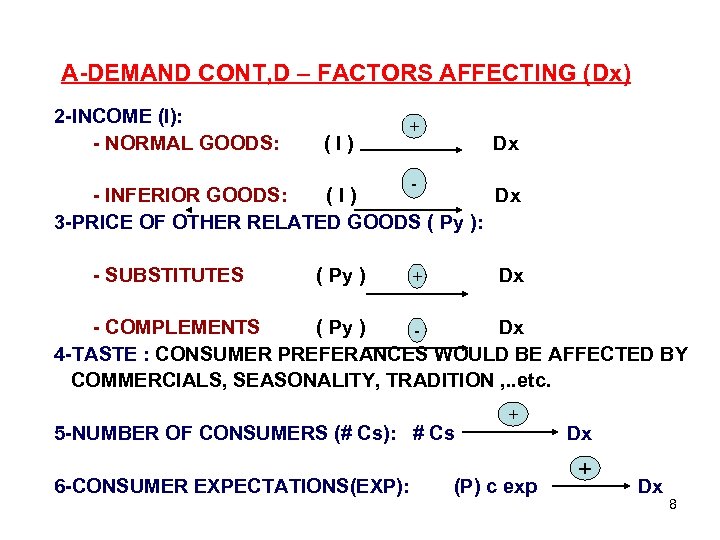
A-DEMAND CONT, D – FACTORS AFFECTING (Dx) 2 -INCOME (I): - NORMAL GOODS: (I) + Dx - - INFERIOR GOODS: (I) Dx 3 -PRICE OF OTHER RELATED GOODS ( Py ): - SUBSTITUTES ( Py ) Dx + - COMPLEMENTS ( Py ) Dx 4 -TASTE : CONSUMER PREFERANCES WOULD BE AFFECTED BY COMMERCIALS, SEASONALITY, TRADITION , . . etc. 5 -NUMBER OF CONSUMERS (# Cs): # Cs 6 -CONSUMER EXPECTATIONS(EXP): + (P) c exp Dx + Dx 8

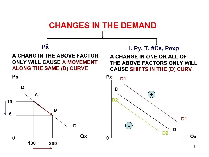
CHANGES IN THE DEMAND Px I, Py, T, #Cs, Pexp A CHANG IN THE ABOVE FACTOR ONLY WILL CAUSE A MOVEMENT ALONG THE SAME (D) CURVE Px A CHANGE IN ONE OR ALL OF THE ABOVE FACTORS ONLY WILL CAUSE SHIFTS IN THE (D) CURV Px D D 1 D + + A D 2 10 B 6 D 1 - D 0 Qx 100 300 0 D 2 D Qx 9

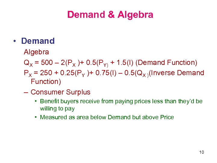
Demand & Algebra • Demand Algebra QX = 500 – 2(PX )+ 0. 5(PY) + 1. 5(I) (Demand Function) PX = 250 + 0. 25(PY )+ 0. 75(I) – 0. 5(QX )(Inverse Demand Function) – Consumer Surplus • Benefit buyers receive from paying prices less than they’d be willing to pay • Measured as area below Demand but above Price 10

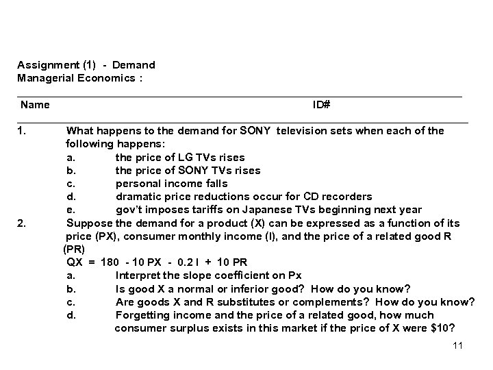
Assignment (1) - Demand Managerial Economics : _____________________________________ Name ID# _____________________________________ 1. What happens to the demand for SONY television sets when each of the following happens: a. the price of LG TVs rises b. the price of SONY TVs rises c. personal income falls d. dramatic price reductions occur for CD recorders e. gov’t imposes tariffs on Japanese TVs beginning next year 2. Suppose the demand for a product (X) can be expressed as a function of its price (PX), consumer monthly income (I), and the price of a related good R (PR) QX = 180 - 10 PX - 0. 2 I + 10 PR a. Interpret the slope coefficient on Px b. Is good X a normal or inferior good? How do you know? c. Are goods X and R substitutes or complements? How do you know? d. Forgetting income and the price of a related good, how much consumer surplus exists in this market if the price of X were $10? 11

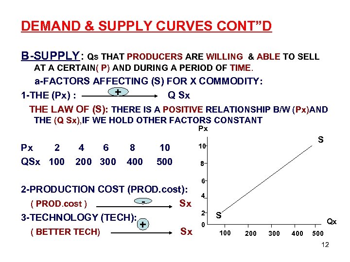
DEMAND & SUPPLY CURVES CONT”D B-SUPPLY: Qs THAT PRODUCERS ARE WILLING & ABLE TO SELL AT A CERTAIN( P) AND DURING A PERIOD OF TIME. a-FACTORS AFFECTING (S) FOR X COMMODITY: + 1 -THE (Px) : Q Sx THE LAW OF (S): THERE IS A POSITIVE RELATIONSHIP B/W (Px)AND THE (Q Sx), IF WE HOLD OTHER FACTORS CONSTANT Px Px 2 QSx 100 4 6 200 300 8 400 10 500 2 -PRODUCTION COST (PROD. cost): ( PROD. cost ) Sx 3 -TECHNOLOGY (TECH): + ( BETTER TECH) Sx S 10 8 6 4 2 S Qx 0 100 200 300 400 500 12

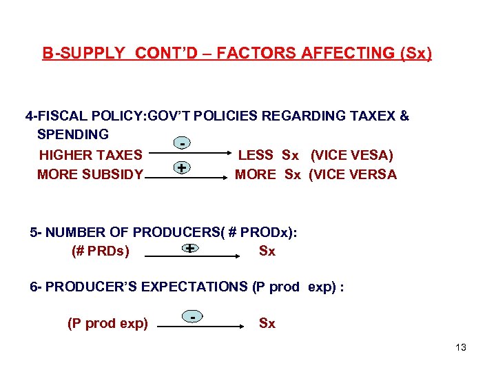
B-SUPPLY CONT’D – FACTORS AFFECTING (Sx) 4 -FISCAL POLICY: GOV’T POLICIES REGARDING TAXEX & SPENDING HIGHER TAXES MORE SUBSIDY + LESS Sx (VICE VESA) MORE Sx (VICE VERSA 5 - NUMBER OF PRODUCERS( # PRODx): + (# PRDs) Sx 6 - PRODUCER’S EXPECTATIONS (P prod exp) : (P prod exp) - Sx 13

CHANGES IN THE SUPPLY COST, Py, TECH. , #Ps, Pexp, FISCAL POLICY Px A CHANGE IN ONE OR ALL OF THE ABOVE FACTORS ONLY WILL CAUSE SHIFTS IN THE (S) CURV A CHANG IN THE ABOVE FACTOR ONLY WILL CAUSE A MOVEMENT ALONG THE SAME (S) CURVE Px Px s 2 S - S S 1 A 10 s 1 B 6 + S 0 S Qx 300 500 S 1 0 Qx 14

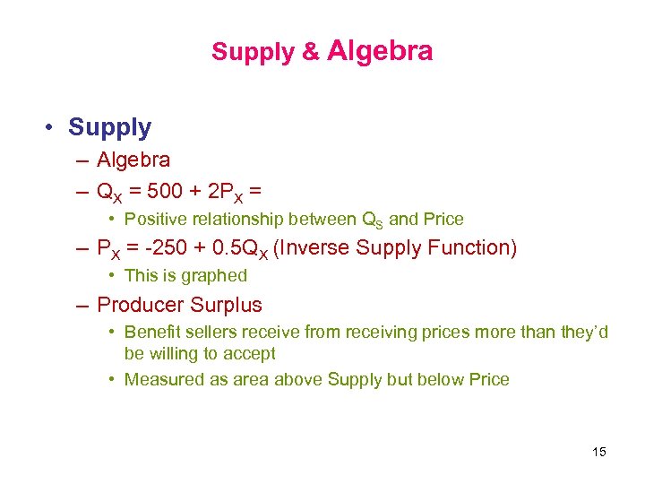
Supply & Algebra • Supply – Algebra – QX = 500 + 2 PX = • Positive relationship between QS and Price – PX = -250 + 0. 5 QX (Inverse Supply Function) • This is graphed – Producer Surplus • Benefit sellers receive from receiving prices more than they’d be willing to accept • Measured as area above Supply but below Price 15

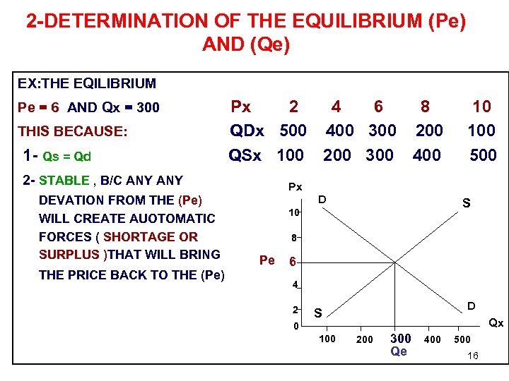
2 -DETERMINATION OF THE EQUILIBRIUM (Pe) AND (Qe) EX: THE EQILIBRIUM Pe = 6 AND Qx = 300 THIS BECAUSE: 1 - Qs = Qd Px 2 4 6 8 QDx 500 400 300 200 QSx 100 200 300 400 2 - STABLE , B/C ANY DEVATION FROM THE (Pe) WILL CREATE AUOTOMATIC FORCES ( SHORTAGE OR SURPLUS )THAT WILL BRING THE PRICE BACK TO THE (Pe) 10 100 500 Px D S 10 8 Pe 6 4 2 D S Qx 0 100 200 300 Qe 400 500 16

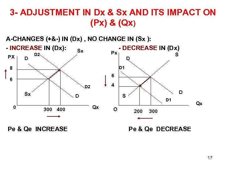
3 - ADJUSTMENT IN Dx & Sx AND ITS IMPACT ON (Px) & (Qx) A-CHANGES (+&-) IN (Dx) , NO CHANGE IN (Sx ): - INCREASE IN (Dx): - DECREASE IN (Dx) Sx PX D Px D 2 S D D 1 8 6 6 4 D 2 Sx 0 D 300 400 Pe & Qe INCREASE D S Qx O D 1 200 Qx 300 Pe & Qe DECREASE 17

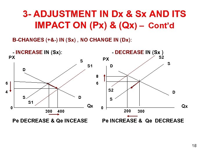
3 - ADJUSTMENT IN Dx & Sx AND ITS IMPACT ON (Px) & (Qx) – Cont’d B-CHANGES (+&-) IN (Sx) , NO CHANGE IN (Dx): - INCREASE IN (Sx): PX - DECREASE IN (Sx ) S S 1 D S 2 PX S D 8 6 6 S 2 4 S D S 1 0 S Qx 300 D 400 Pe DECREASE & Qe INCEASE 0 Qx 200 300 Pe INCREASE & Qe DECREASE 18

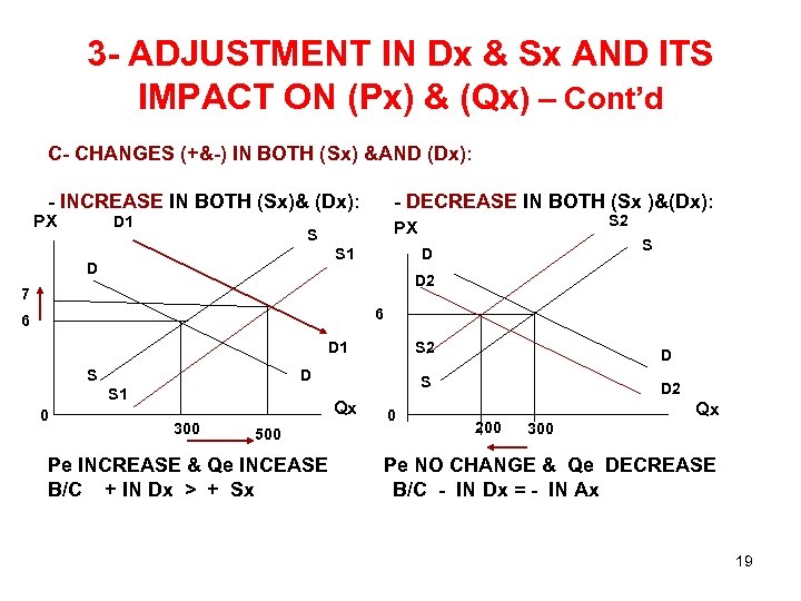
3 - ADJUSTMENT IN Dx & Sx AND ITS IMPACT ON (Px) & (Qx) – Cont’d C- CHANGES (+&-) IN BOTH (Sx) &AND (Dx): - INCREASE IN BOTH (Sx)& (Dx): PX D 1 - DECREASE IN BOTH (Sx )&(Dx): S S 1 D S 2 PX S D D 2 7 6 6 D 1 S Qx 300 500 Pe INCREASE & Qe INCEASE B/C + IN Dx > + Sx 0 D S 1 0 S 2 D 2 Qx 200 300 Pe NO CHANGE & Qe DECREASE B/C - IN Dx = - IN Ax 19

4 - GOV’T. INTERVENTION IN MARKETS: A-PRICE CEILING : CAUSE SHORTAGE (AB) B- PRICE FLOOR: CAUSE SURPLUS(CD) Px Px D S A 0 D D S Qx 200 300 400 e 6 B S D C Pf 8 e 6 Pc 4 S D 0 200 300 400 Qx 20

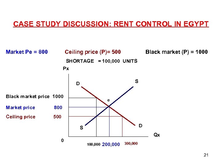
CASE STUDY DISCUSSION: RENT CONTROL IN EGYPT Market Pe = 800 Ceiling price (P)= 500 Black market (P) = 1000 SHORTAGE = 100, 000 UNITS Px S D Black market price 1000 Market price 800 Ceiling price e 500 D S Qx 0 100, 000 200, 000 300, 000 21

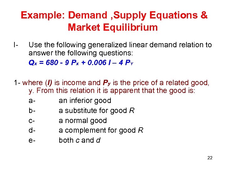
Example: Demand , Supply Equations & Market Equilibrium I- Use the following generalized linear demand relation to answer the following questions: Qx = 680 - 9 Px + 0. 006 I – 4 PY 1 - where (I) is income and Py is the price of a related good, y. From this relation it is apparent that the good is: aan inferior good ba substitute for good R ca normal good da complement for good R eboth c and d 22

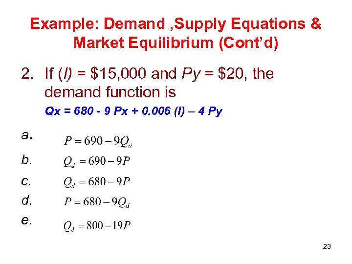
Example: Demand , Supply Equations & Market Equilibrium (Cont’d) 2. If (I) = $15, 000 and Py = $20, the demand function is Qx = 680 - 9 Px + 0. 006 (I) – 4 Py a. b. c. d. e. 23

3. If (I) = $15, 000 and Py = $20 and the supply function is Qx = 30 + 3 Px , equilibrium price and quantity are, respectively, a. b. c. d. e. P = $55 and Q = 195. P = $9 and Q = 609. P = $12 and Q = 200. P = $50 and Q = 170. P = $40 and Q = 250. 24

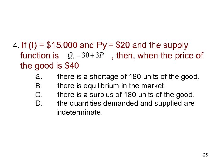
4. If (I) = $15, 000 and Py = $20 and the supply function is , then, when the price of the good is $40 a. there is a shortage of 180 units of the good. B. C. D. there is equilibrium in the market. there is a surplus of 180 units of the good. the quantities demanded and supplied are indeterminate. 25

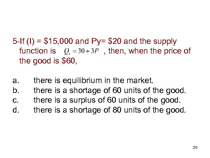
5 -If (I) = $15, 000 and Py= $20 and the supply function is , then, when the price of the good is $60, a. b. c. d. there is equilibrium in the market. there is a shortage of 60 units of the good. there is a surplus of 60 units of the good. there is a shortage of 80 units of the good. 26

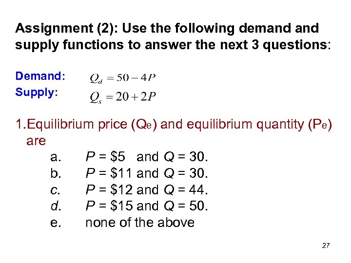
Assignment (2): Use the following demand supply functions to answer the next 3 questions: Demand: Supply: 1. Equilibrium price (Qe) and equilibrium quantity (Pe) are a. P = $5 and Q = 30. b. P = $11 and Q = 30. c. P = $12 and Q = 44. d. P = $15 and Q = 50. e. none of the above 27

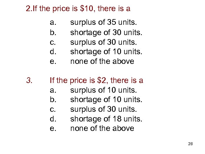
2. If the price is $10, there is a a. b. c. d. e. 3. surplus of 35 units. shortage of 30 units. surplus of 30 units. shortage of 10 units. none of the above If the price is $2, there is a a. surplus of 10 units. b. shortage of 10 units. c. surplus of 30 units. d. shortage of 18 units. e. none of the above 28

(4) : Answer The Following Questions - Assume that the equilibrium price of Nokia mobile brand name (x) Pe =1000 and equilibrium quantity Qe = 400 , show this graphically. what will happen if the price of the Samsung mobile brand name -Y increases and the cost of producing the Nokia mobile increased by the same percentage (Hint : Make shift in D =shift in S) 29

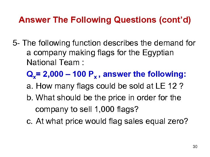
Answer The Following Questions (cont’d) 5 - The following function describes the demand for a company making flags for the Egyptian National Team : Qx= 2, 000 – 100 Px , answer the following: a. How many flags could be sold at LE 12 ? b. What should be the price in order for the company to sell 1, 000 flags? c. At what price would flag sales equal zero? 30

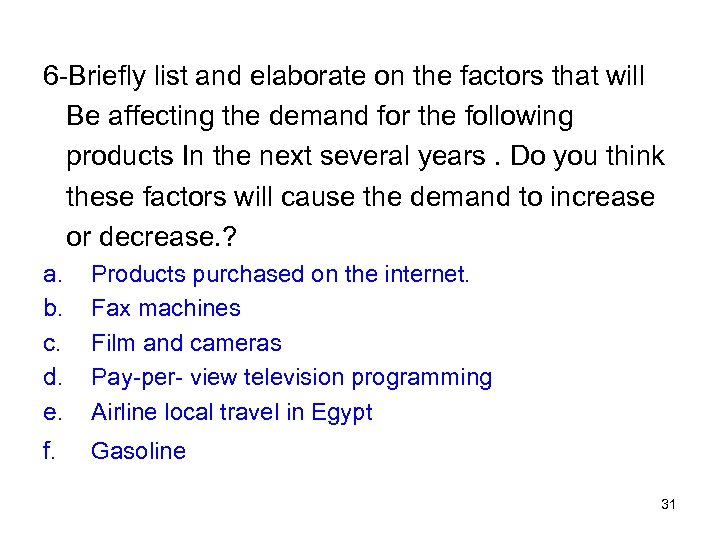
6 -Briefly list and elaborate on the factors that will Be affecting the demand for the following products In the next several years. Do you think these factors will cause the demand to increase or decrease. ? a. b. c. d. e. Products purchased on the internet. Fax machines Film and cameras Pay-per- view television programming Airline local travel in Egypt f. Gasoline 31

7 -Briefly list and elaborate on the factors that will Be affecting the supply for the following products In the next several years. Do you think these factors will cause the supply to increase or decrease. ? a. b. c. d. e. f. Crude oil Beef Computer memory chips Hotel rooms Laptop computers Credit cards issued by financial institutions 32

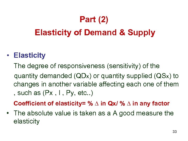
Part (2) Elasticity of Demand & Supply • Elasticity The degree of responsiveness (sensitivity) of the quantity demanded (QDx) or quantity supplied (QSx) to changes in another variable affecting each one of them , such as (Px , I , Py, etc. . ) Coefficient of elasticity= % ∆ in Qx/ % ∆ in any factor • The absolute value is taken as a A good measure the elasticity 33

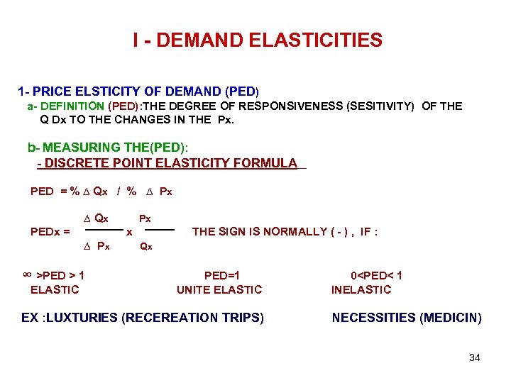
I - DEMAND ELASTICITIES 1 - PRICE ELSTICITY OF DEMAND (PED) a- DEFINITION (PED): THE DEGREE OF RESPONSIVENESS (SESITIVITY) OF THE Q Dx TO THE CHANGES IN THE Px. b- MEASURING THE(PED): - DISCRETE POINT ELASTICITY FORMULA PED = % ∆ Qx / % ∆ Px ∆ Qx PEDx = x ∆ Px ∞ >PED > 1 ELASTIC Px THE SIGN IS NORMALLY ( - ) , IF : Qx PED=1 UNITE ELASTIC EX : LUXTURIES (RECEREATION TRIPS) 0

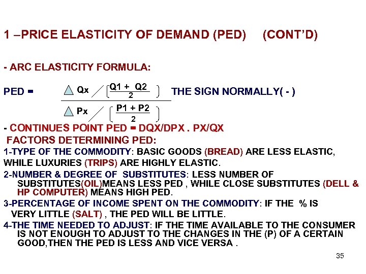
1 –PRICE ELASTICITY OF DEMAND (PED) (CONT’D) - ARC ELASTICITY FORMULA: Qx Q 1 + Q 2 Px PED = P 1 + P 2 2 THE SIGN NORMALLY( - ) 2 - CONTINUES POINT PED = DQX/DPX. PX/QX FACTORS DETERMINING PED: 1 -TYPE OF THE COMMODITY: BASIC GOODS (BREAD) ARE LESS ELASTIC, WHILE LUXURIES (TRIPS) ARE HIGHLY ELASTIC. 2 -NUMBER & DEGREE OF SUBSTITUTES: LESS NUMBER OF SUBSTITUTES(OIL)MEANS LESS PED , WHILE CLOSE SUBSTITUTES (DELL & HP COMPUTER) MEANS HIGH PED. 3 -PERCENTAGE OF INCOME SPENT ON THE COMMODITY: IF THE % IS VERY LITTLE (SALT) , THE PED WILL BE LITTLE. 4 -THE TIME NEEDED TO ADJUST: IF THE TIME AVAILABLE TO THE CONSUMER IS NOT ENOUGH TO ADJUST TO THE CHANGES IN THE (P) OF A CERTAIN GOOD, THEN THE PED IS LESS AND VICE VERSA. 35

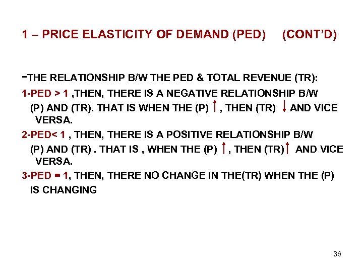
1 – PRICE ELASTICITY OF DEMAND (PED) (CONT’D) -THE RELATIONSHIP B/W THE PED & TOTAL REVENUE (TR): 1 -PED > 1 , THEN, THERE IS A NEGATIVE RELATIONSHIP B/W (P) AND (TR). THAT IS WHEN THE (P) , THEN (TR) AND VICE VERSA. 2 -PED< 1 , THEN, THERE IS A POSITIVE RELATIONSHIP B/W (P) AND (TR). THAT IS , WHEN THE (P) , THEN (TR) AND VICE VERSA. 3 -PED = 1, THEN, THERE NO CHANGE IN THE(TR) WHEN THE (P) IS CHANGING 36

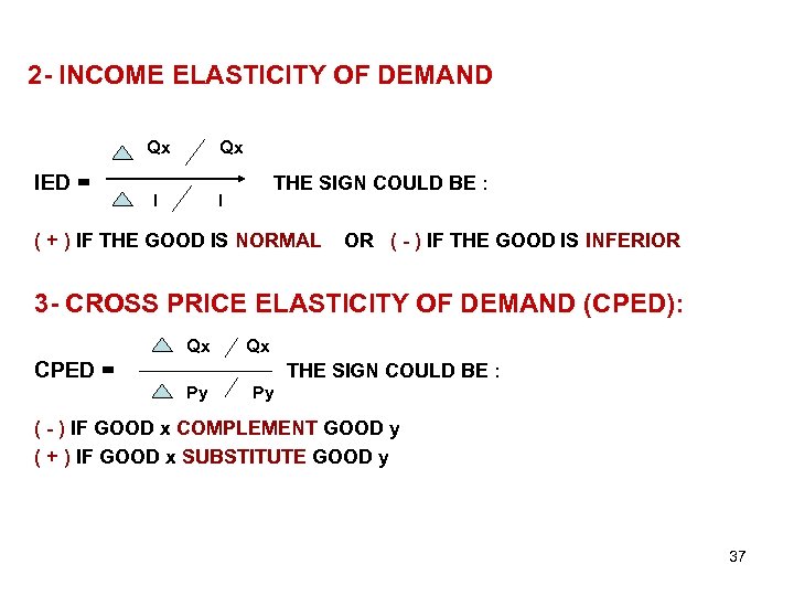
2 - INCOME ELASTICITY OF DEMAND Qx IED = Qx I THE SIGN COULD BE : I ( + ) IF THE GOOD IS NORMAL OR ( - ) IF THE GOOD IS INFERIOR 3 - CROSS PRICE ELASTICITY OF DEMAND (CPED): Qx Qx CPED = THE SIGN COULD BE : Py Py ( - ) IF GOOD x COMPLEMENT GOOD y ( + ) IF GOOD x SUBSTITUTE GOOD y 37

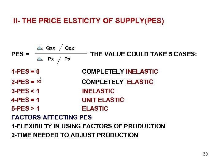
II- THE PRICE ELSTICITY OF SUPPLY(PES) Qsx PES = 1 -PES = 0 Px Qsx Px THE VALUE COULD TAKE 5 CASES: COMPLETELY INELASTIC 2 -PES = ∞ COMPLETELY ELASTIC 3 -PES < 1 INELASTIC 4 -PES = 1 UNIT ELASTIC 5 -PES > 1 ELASTIC FACTORS AFFECTING PES 1 -FLEXIBILTY IN USING FACTORS OF PRODUCTION 2 -TIME NEEDED TO ADJUST PRODUCTION 38

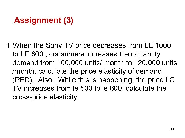
Assignment (3) 1 -When the Sony TV price decreases from LE 1000 to LE 800 , consumers increases their quantity demand from 100, 000 units/ month to 120, 000 units /month. calculate the price elasticity of demand (PED). Also , While this is happening, the price LG TV increases from le 500 to le 600, calculate the cross-price elasticity. 39

Answer the Following Questions 2 - Discuss the relative (PED) of the following products: a. Mayonnaise b. Chevrolet automobiles c. Washing machines d. Air travel (vacation) e. Diamond rings 3 - Would you expect the (CPED) coefficient b/w each of the following pairs of products to be (+) or (-) a. Personal computers and software. b. Electricity and natural gas c. Bread and CDs 40

Answer the Following Questions 4 - Discuss the (IED) of the following consumer products: a. Fine Jewelry b. Studio apartments c. Fool and Falafel sandwiches d. Riding microbus e. Salt 5 - The equation for a demand curve has been estimated to be : Qx = 100 – 10 Px + 0. 5 (I). Assume Px = 7 and (I) = 50. a. Interpret the equation. b. At a Px = 7, what is the PED? c. At an income of 50, what is IED? d. Now assume (I) = 70, what is the PED at Px = 8 ? 41

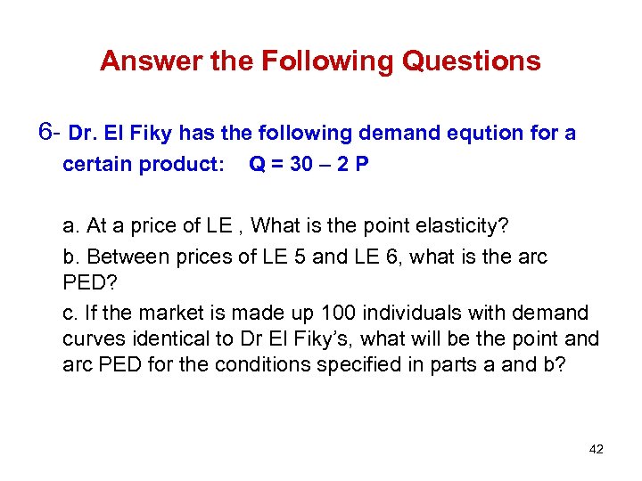
Answer the Following Questions 6 - Dr. El Fiky has the following demand eqution for a certain product: Q = 30 – 2 P a. At a price of LE , What is the point elasticity? b. Between prices of LE 5 and LE 6, what is the arc PED? c. If the market is made up 100 individuals with demand curves identical to Dr El Fiky’s, what will be the point and arc PED for the conditions specified in parts a and b? 42

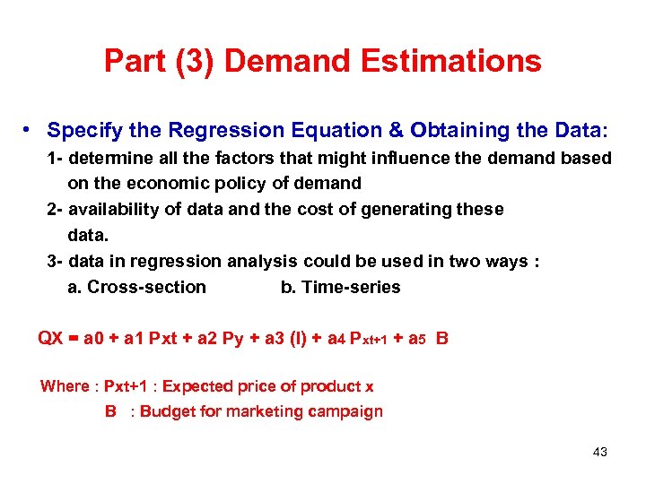
Part (3) Demand Estimations • Specify the Regression Equation & Obtaining the Data: 1 - determine all the factors that might influence the demand based on the economic policy of demand 2 - availability of data and the cost of generating these data. 3 - data in regression analysis could be used in two ways : a. Cross-section b. Time-series QX = a 0 + a 1 Pxt + a 2 Py + a 3 (I) + a 4 Pxt+1 + a 5 B Where : Pxt+1 : Expected price of product x B : Budget for marketing campaign 43

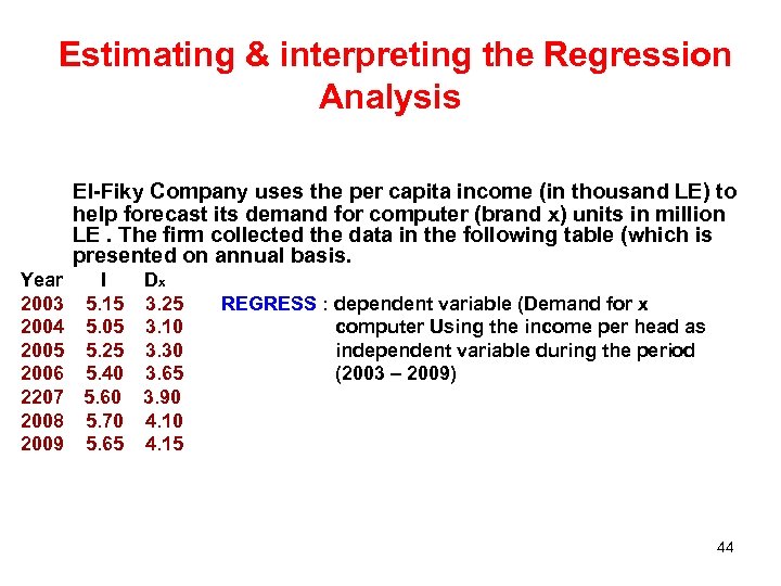
Estimating & interpreting the Regression Analysis El-Fiky Company uses the per capita income (in thousand LE) to help forecast its demand for computer (brand x) units in million LE. The firm collected the data in the following table (which is presented on annual basis. Year I Dx 2003 5. 15 3. 25 2004 5. 05 3. 10 2005 5. 25 3. 30 2006 5. 40 3. 65 2207 5. 60 3. 90 2008 5. 70 4. 10 2009 5. 65 4. 15 REGRESS : dependent variable (Demand for x computer Using the income per head as independent variable during the period (2003 – 2009) 44

Variable Coefficient Std Err T-stat CONST (I) -5. 20679 0. 616404 -8. 44704 1. 63750 0. 114037 14. 3594 No. of Observations = 7 R² =. 9763 (adj)=. 9716 Sum of Sq. Resid. =. 260089 E-01 Std. Error of Reg. =. 721234 E-01 Durbin-Watson = 2. 0012 F ( 1, 5) = 206. 191 Significance =. 05 45

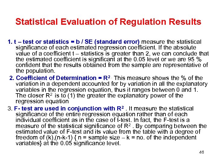
Statistical Evaluation of Regulation Results 1. t – test or statistics = b / SE (standard error) measure the statistical significance of each estimated regression coefficient. If the absolute value of a coefficient t – statistics is greater than 2, we can conclude that the estimated coefficient is significant at the 0. 05 level or we are 95 % confident that the results obtained from the sample are representative of the population. 2. Coefficient of Determination = R 2. This measure shows the % of the variation in a dependent accounted for by variation in all the explanatory variables in the regression equation, thus it ranges between 0 and 1. The closer R 2 is to (1) the greater the explanatory power of the regression equation 3. F- test are used in conjunction with R 2. It measure the statistical significance of the entire regression equation rather than of each individual coefficient as in the case of t-test. In fact, the F-test is a measure of the statistical significance of R 2. By comparing between the estimated value of F-test and its value from the table with a degree of freedom of (k), (n-k-1) { n = sample size – k = no. of the independent variables} at the 0. 05 significance level. 46

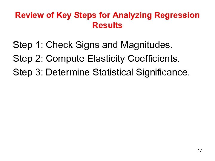
Review of Key Steps for Analyzing Regression Results Step 1: Check Signs and Magnitudes. Step 2: Compute Elasticity Coefficients. Step 3: Determine Statistical Significance. 47

Problems in The Use of Regression Analysis 1 - The Identification Problem 2 - Multicollinearity 3 - Auto correlation 48

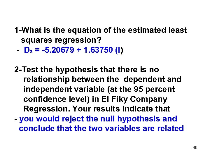
1 -What is the equation of the estimated least squares regression? - Dx = -5. 20679 + 1. 63750 (I) 2 -Test the hypothesis that there is no relationship between the dependent and independent variable (at the 95 percent confidence level) in El Fiky Company Regression. Your results indicate that - you would reject the null hypothesis and conclude that the two variables are related 49

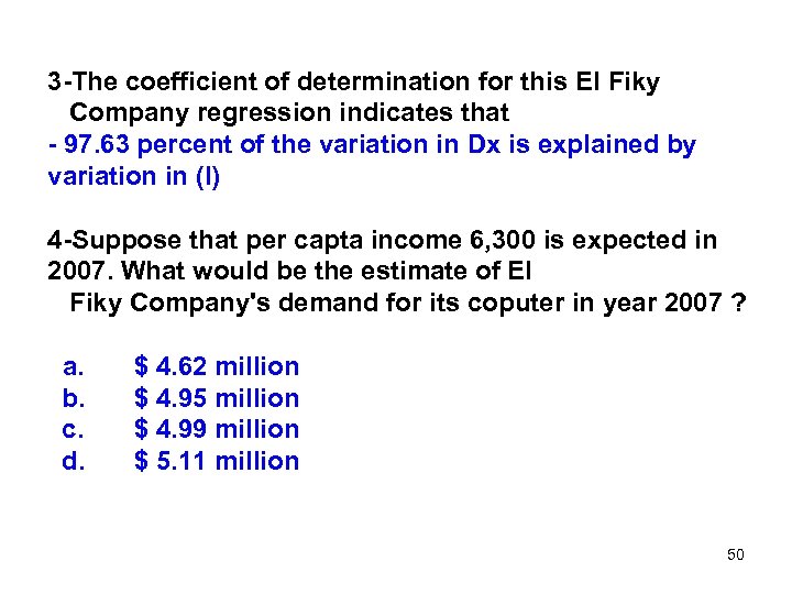
3 -The coefficient of determination for this El Fiky Company regression indicates that - 97. 63 percent of the variation in Dx is explained by variation in (I) 4 -Suppose that per capta income 6, 300 is expected in 2007. What would be the estimate of El Fiky Company's demand for its coputer in year 2007 ? a. b. c. d. $ 4. 62 million $ 4. 95 million $ 4. 99 million $ 5. 11 million 50

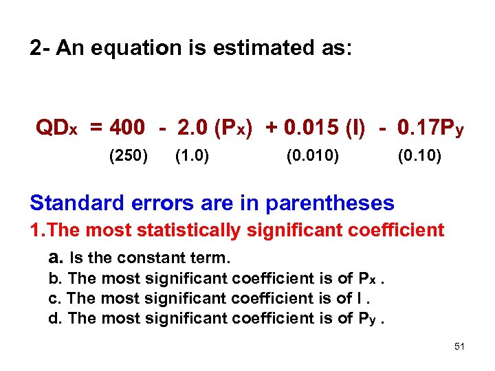
2 - An equation is estimated as: QDx = 400 - 2. 0 (Px) + 0. 015 (I) - 0. 17 Py (250) (1. 0) (0. 010) (0. 10) Standard errors are in parentheses 1. The most statistically significant coefficient a. Is the constant term. b. The most significant coefficient is of Px. c. The most significant coefficient is of I. d. The most significant coefficient is of Py. 51

2 -The statistic used to test whether the independent variables taken as group statistically explain variation in the dependent variable is the a. R-squared statistic. b. t-statistic. c. Durbin-Watson statistic. d. F-test statistic. 3 - Serial correlation occurs when a. independent variables are correlated across observations. b. dependent variables are correlated across observations. c. error terms are correlated across observations. d. R-squared is near one and the t-statistics are near zero. 52

4 -The statistic that tests an individual coefficient for statistical significance is the a. R-squared statistic. b. t-statistic. c. Durbin-Watson statistic. d. F-test statistic. 5 - Multiple regression differs from simple regression in that a. there can be multiple dependent variables. b. the time periods over which observations are taken are multiplied to increase explanatory power. c. a simple regression is done multiple times to increase explanatory power. d. there are multiple independent variables. 53

Part (4): Forecasting • Forecast helps in two areas: 1 - Setting cos. Objectives. Revenue or profit Growth- return on investment 2 - Constructing cos. business plans. company planners in all areas; sales, HR, facilities, manufacturing, finance , will utilize an array of forecast in constructing the various portions of the plan • Subjects of Forecast: 1 - Macroeconomic Level 2 - Sector level 3 - Industry level 4 - Product level 54

Demand Estimate & Forecasting • Prerequisite of a good forecast 1 - Consistency with other parts of the business. 2 - Adequate knowledge of the relevant past. 3 - Take into consideration the econ. & political environment. 4 - Conducted in timely fashion 55

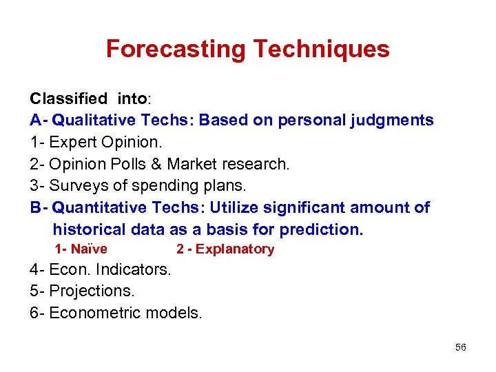
Forecasting Techniques Classified into: A- Qualitative Techs: Based on personal judgments 1 - Expert Opinion. 2 - Opinion Polls & Market research. 3 - Surveys of spending plans. B- Quantitative Techs: Utilize significant amount of historical data as a basis for prediction. 1 - Naïve 2 - Explanatory 4 - Econ. Indicators. 5 - Projections. 6 - Econometric models. 56

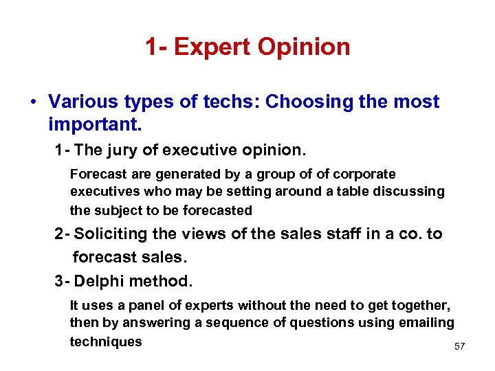
1 - Expert Opinion • Various types of techs: Choosing the most important. 1 - The jury of executive opinion. Forecast are generated by a group of of corporate executives who may be setting around a table discussing the subject to be forecasted 2 - Soliciting the views of the sales staff in a co. to forecast sales. 3 - Delphi method. It uses a panel of experts without the need to get together, then by answering a sequence of questions using emailing techniques 57

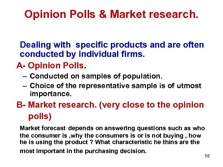
Opinion Polls & Market research. Dealing with specific products and are often conducted by individual firms. A- Opinion Polls. – Conducted on samples of population. – Choice of the representative sample is of utmost importance. B- Market research. (very close to the opinion polls) Market forecast depends on answering questions such as who the consumer is , why the consumers is or is not buying , how he is using the product ? What characteristic he thins are the most important in the purchasing decision. 58

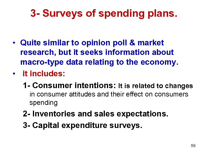
3 - Surveys of spending plans. • Quite similar to opinion poll & market research, but it seeks information about macro-type data relating to the economy. • it includes: 1 - Consumer intentions: It is related to changes in consumer attitudes and their effect on consumers spending 2 - Inventories and sales expectations. 3 - Capital expenditure surveys. 59

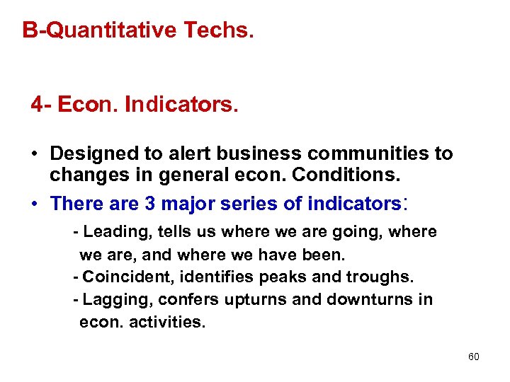
B-Quantitative Techs. 4 - Econ. Indicators. • Designed to alert business communities to changes in general econ. Conditions. • There are 3 major series of indicators: - Leading, tells us where we are going, where we are, and where we have been. - Coincident, identifies peaks and troughs. - Lagging, confers upturns and downturns in econ. activities. 60

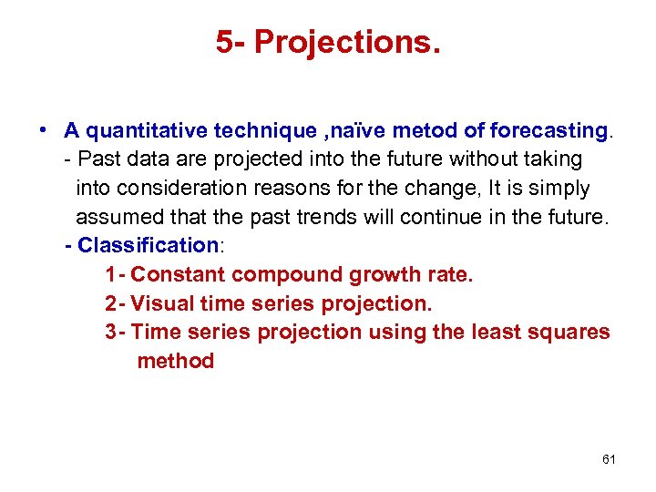
5 - Projections. • A quantitative technique , naïve metod of forecasting. - Past data are projected into the future without taking into consideration reasons for the change, It is simply assumed that the past trends will continue in the future. - Classification: 1 - Constant compound growth rate. 2 - Visual time series projection. 3 - Time series projection using the least squares method 61

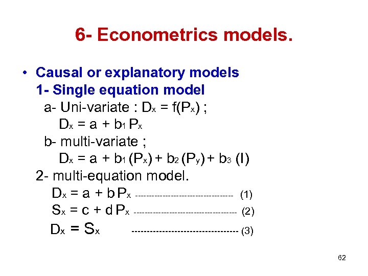
6 - Econometrics models. • Causal or explanatory models 1 - Single equation model a- Uni-variate : Dx = f(Px) ; Dx = a + b 1 P x b- multi-variate ; Dx = a + b 1 (Px) + b 2 (Py) + b 3 (I) 2 - multi-equation model. Dx = a + b Px ------------------ (1) Sx = c + d Px ------------------- (2) Dx = S x ------------------ (3) 62

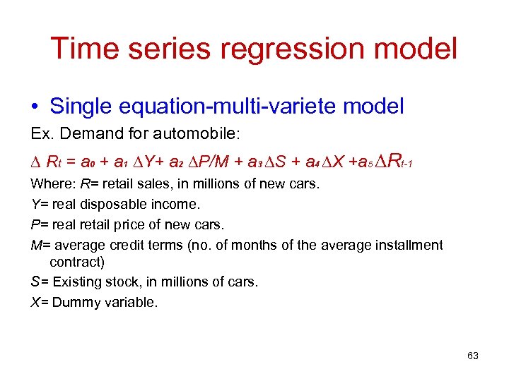
Time series regression model • Single equation-multi-variete model Ex. Demand for automobile: ∆ Rt = a 0 + a 1 ∆Y+ a 2 ∆P/M + a 3 ∆S + a 4 ∆X +a 5 ∆Rt-1 Where: R= retail sales, in millions of new cars. Y= real disposable income. P= real retail price of new cars. M= average credit terms (no. of months of the average installment contract) S= Existing stock, in millions of cars. X= Dummy variable. 63

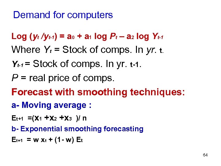
Demand for computers Log (yt /yt-1) = a 0 + a 1 log Pt – a 2 log Yt-1 Where Yt = Stock of comps. In yr. t. Yt-1 = Stock of comps. In yr. t-1. P = real price of comps. Forecast with smoothing techniques: a- Moving average : Et+1 =(x 1 +x 2 +x 3 )/ n b- Exponential smoothing forecasting Et+1 = w xt + (1 - w) Et 64

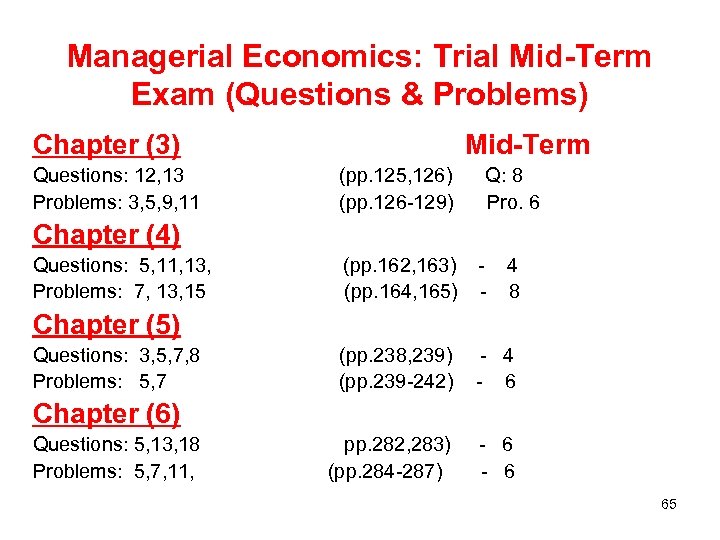
Managerial Economics: Trial Mid-Term Exam (Questions & Problems) Chapter (3) Questions: 12, 13 Problems: 3, 5, 9, 11 Mid-Term (pp. 125, 126) (pp. 126 -129) Q: 8 Pro. 6 Chapter (4) Questions: 5, 11, 13, Problems: 7, 13, 15 (pp. 162, 163) (pp. 164, 165) - 4 8 (pp. 238, 239) (pp. 239 -242) - 4 - 6 pp. 282, 283) (pp. 284 -287) - 6 Chapter (5) Questions: 3, 5, 7, 8 Problems: 5, 7 Chapter (6) Questions: 5, 13, 18 Problems: 5, 7, 11, 65

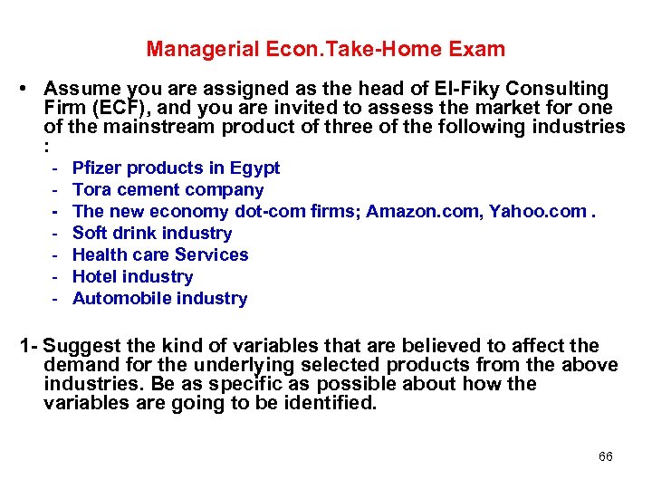
Managerial Econ. Take-Home Exam • Assume you are assigned as the head of El-Fiky Consulting Firm (ECF), and you are invited to assess the market for one of the mainstream product of three of the following industries : - Pfizer products in Egypt Tora cement company The new economy dot-com firms; Amazon. com, Yahoo. com. Soft drink industry Health care Services Hotel industry Automobile industry 1 - Suggest the kind of variables that are believed to affect the demand for the underlying selected products from the above industries. Be as specific as possible about how the variables are going to be identified. 66

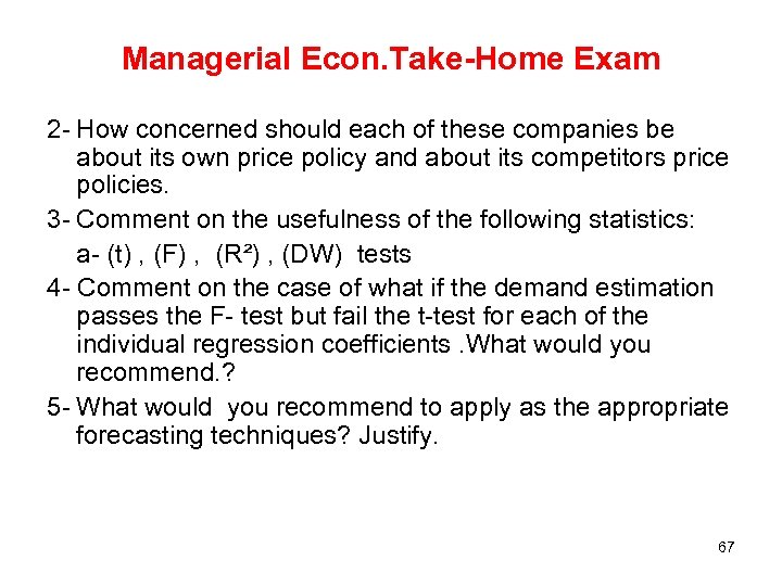
Managerial Econ. Take-Home Exam 2 - How concerned should each of these companies be about its own price policy and about its competitors price policies. 3 - Comment on the usefulness of the following statistics: a- (t) , (F) , (R²) , (DW) tests 4 - Comment on the case of what if the demand estimation passes the F- test but fail the t-test for each of the individual regression coefficients. What would you recommend. ? 5 - What would you recommend to apply as the appropriate forecasting techniques? Justify. 67

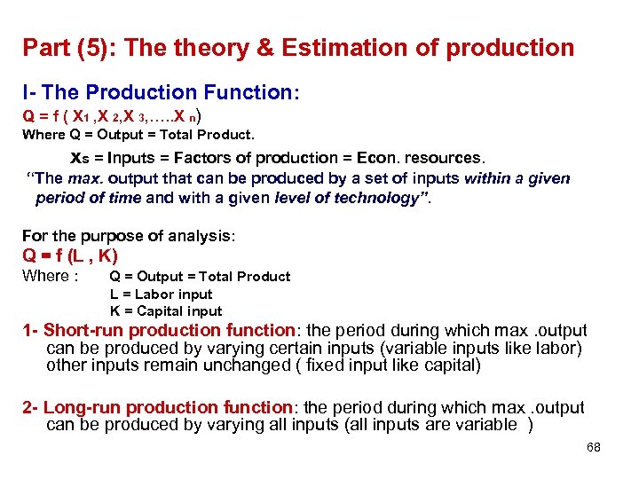
Part (5): The theory & Estimation of production I- The Production Function: Q = f ( X 1 , X 2, X 3, …. . X n) Where Q = Output = Total Product. xs = Inputs = Factors of production = Econ. resources. “The max. output that can be produced by a set of inputs within a given period of time and with a given level of technology”. For the purpose of analysis: Q = f (L , K) Where : Q = Output = Total Product L = Labor input K = Capital input 1 - Short-run production function: the period during which max. output can be produced by varying certain inputs (variable inputs like labor) other inputs remain unchanged ( fixed input like capital) 2 - Long-run production function: the period during which max. output can be produced by varying all inputs (all inputs are variable ) 68

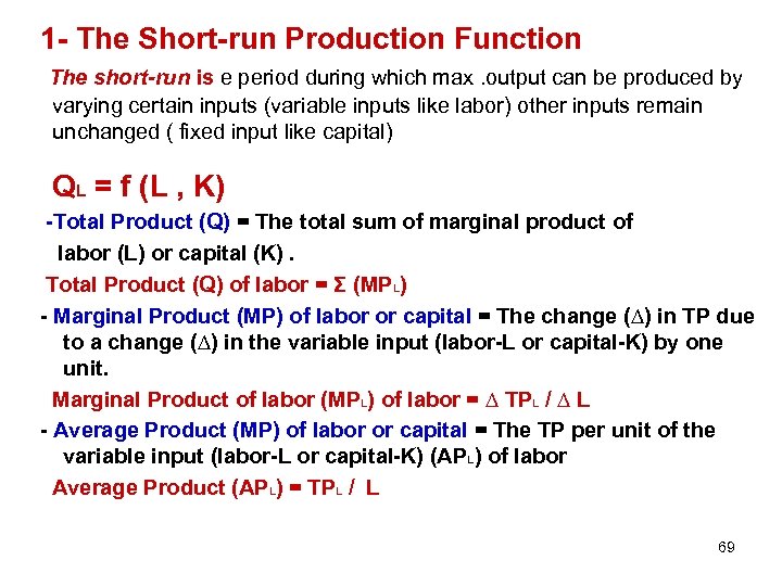
1 - The Short-run Production Function The short-run is e period during which max. output can be produced by varying certain inputs (variable inputs like labor) other inputs remain unchanged ( fixed input like capital) QL = f (L , K) -Total Product (Q) = The total sum of marginal product of labor (L) or capital (K). Total Product (Q) of labor = Σ (MPL) - Marginal Product (MP) of labor or capital = The change (∆) in TP due to a change (∆) in the variable input (labor-L or capital-K) by one unit. Marginal Product of labor (MPL) of labor = ∆ TPL / ∆ L - Average Product (MP) of labor or capital = The TP per unit of the variable input (labor-L or capital-K) (APL) of labor Average Product (APL) = TPL / L 69

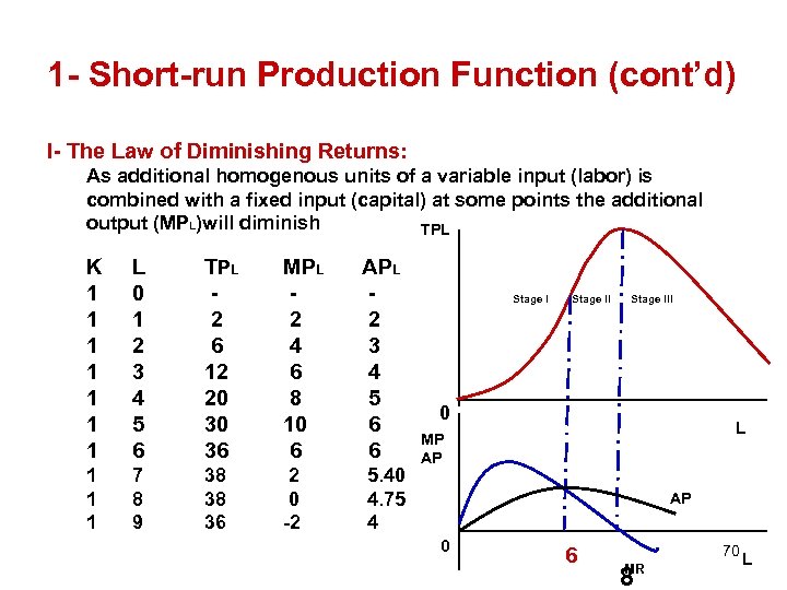
1 - Short-run Production Function (cont’d) I- The Law of Diminishing Returns: As additional homogenous units of a variable input (labor) is combined with a fixed input (capital) at some points the additional output (MPL)will diminish TPL K 1 1 1 1 L 0 1 2 3 4 5 6 TPL 2 6 12 20 30 36 MPL 2 4 6 8 10 6 APL 2 3 4 5 6 6 1 1 1 7 8 9 38 38 36 2 0 -2 5. 40 4. 75 4 Stage III 0 L MP AP AP 0 6 70 MR 8 L

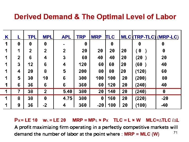
Derived Demand & The Optimal Level of Labor K 1 1 1 1 1 L 0 1 2 3 4 5 6 7 8 9 TPL 0 2 6 12 20 30 36 38 38 36 PX = LE 10 MPL 0 2 4 6 8 10 6 2 0 -2 APL TRP MRP 0 2 20 20 3 60 40 4 120 60 5 200 80 6 300 100 6 360 60 5. 40 380 20 4. 75 380 0 4 360 -20 w. L = LE 20 TLC 0 20 40 60 80 100 120 140 160 180 MLC (TRP-TLC) (MRP-LC) 0 0 20 (0 ) 0 20 (20 ) 20 20 (60 ) 40 20 (120) 60 20 (200) 80 20 (240) 40 20 (240) 0 20 (220) -20 20 (180) -40 MRP = MPL × PX TLC = L × W MLC=∆TLC /∆L A profit maximizing firm operating in a perfectly competitive markets will 71 demand the number of labor at the point where : MRP = MLC (W)

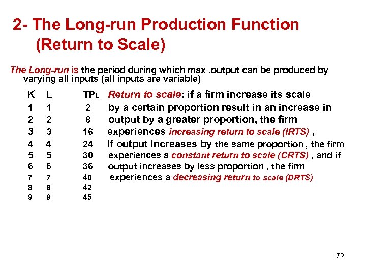
2 - The Long-run Production Function (Return to Scale) The Long-run is the period during which max. output can be produced by varying all inputs (all inputs are variable) K L 1 2 4 5 6 1 2 3 4 5 6 7 8 9 3 TPL Return to scale: if a firm increase its scale 2 by a certain proportion result in an increase in 8 output by a greater proportion, the firm 16 experiences increasing return to scale (IRTS) , 24 if output increases by the same proportion , the firm 30 36 40 42 45 experiences a constant return to scale (CRTS) , and if output increases by less proportion , the firm experiences a decreasing return to scale (DRTS) 72

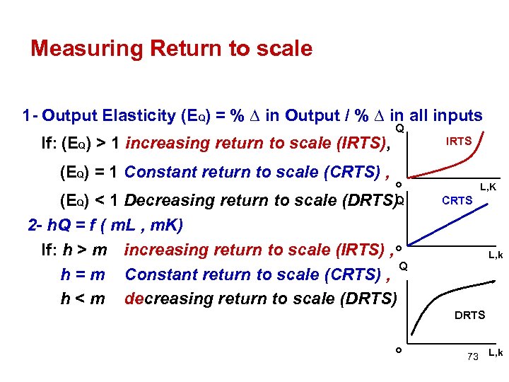
Measuring Return to scale 1 - Output Elasticity (EQ) = % ∆ in Output / % ∆ in all inputs If: (EQ) > 1 increasing return to scale (IRTS), (EQ) = 1 Constant return to scale (CRTS) , Q IRTS o (EQ) < 1 Decreasing return to scale (DRTS)Q 2 - h. Q = f ( m. L , m. K) If: h > m increasing return to scale (IRTS) , o Q h = m Constant return to scale (CRTS) , h < m decreasing return to scale (DRTS) L, K CRTS L, k DRTS o 73 L, k

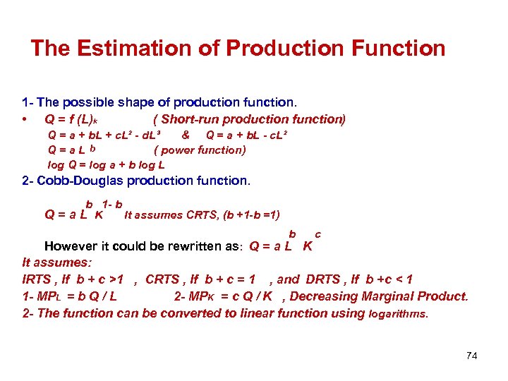
The Estimation of Production Function 1 - The possible shape of production function. • Q = f (L)k ( Short-run production function) Q = a + b. L + c. L² - d. L³ & Q = a + b. L - c. L² Q=a. L b ( power function) log Q = log a + b log L 2 - Cobb-Douglas production function. b 1 - b Q=a. L K It assumes CRTS, (b +1 -b =1) b c However it could be rewritten as: Q = a L K It assumes: IRTS , If b + c >1 , CRTS , If b + c = 1 , and DRTS , If b +c < 1 1 - MPL = b Q / L 2 - MPK = c Q / K , Decreasing Marginal Product. 2 - The function can be converted to linear function using logarithms. 74

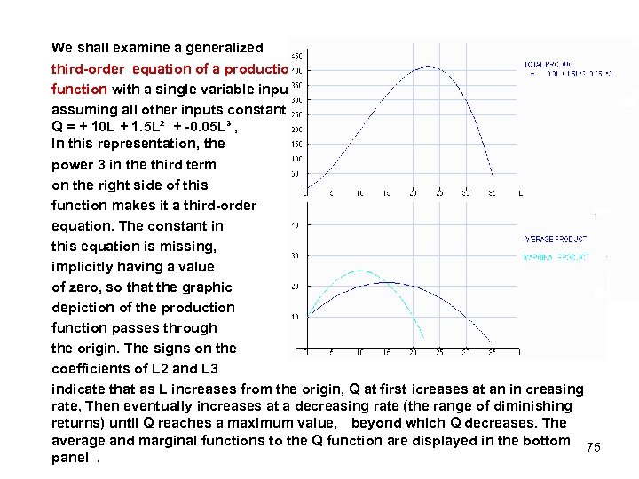
We shall examine a generalized third-order equation of a production function with a single variable input, L, assuming all other inputs constant, Q = + 10 L + 1. 5 L² + -0. 05 L³ , In this representation, the power 3 in the third term on the right side of this function makes it a third-order equation. The constant in this equation is missing, implicitly having a value of zero, so that the graphic depiction of the production function passes through the origin. The signs on the coefficients of L 2 and L 3 indicate that as L increases from the origin, Q at first icreases at an in creasing rate, Then eventually increases at a decreasing rate (the range of diminishing returns) until Q reaches a maximum value, beyond which Q decreases. The average and marginal functions to the Q function are displayed in the bottom 75 panel.

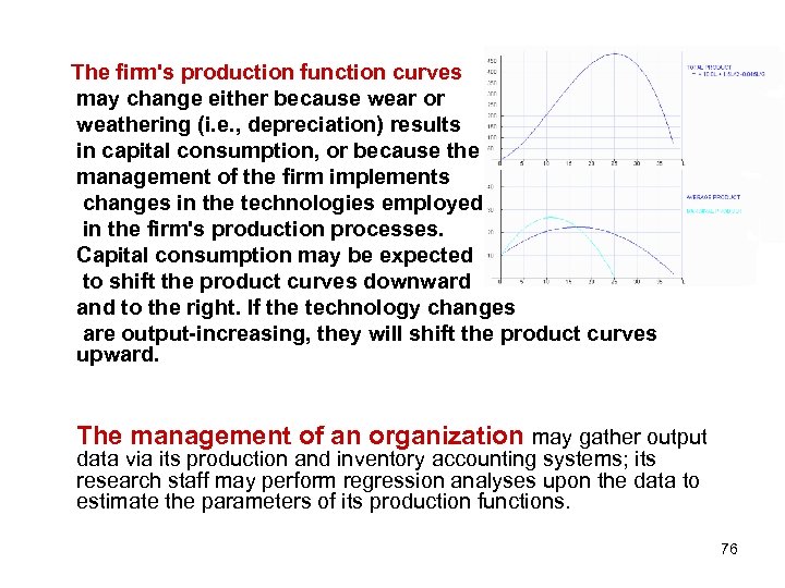
The firm's production function curves may change either because wear or weathering (i. e. , depreciation) results in capital consumption, or because the management of the firm implements changes in the technologies employed in the firm's production processes. Capital consumption may be expected to shift the product curves downward and to the right. If the technology changes are output-increasing, they will shift the product curves upward. The management of an organization may gather output data via its production and inventory accounting systems; its research staff may perform regression analyses upon the data to estimate the parameters of its production functions. 76

Part (5) Problems A firm has the following short-run production function: Q = 50 L +6 L² – 0. 5 L³ a- when does the law of diminishing returns take effect? b- Calculate the values for labor over which stages I , III occur. c- Assume each worker is paid LE 10 per hour and works a 40 hour week, How many workers should the firm hire if the price of the output is LE 10 per unit ? Suppose the price of the output falls to LE 7. 50. What do you think would be the short run impact on the firm’s production ? The long run impact? 77

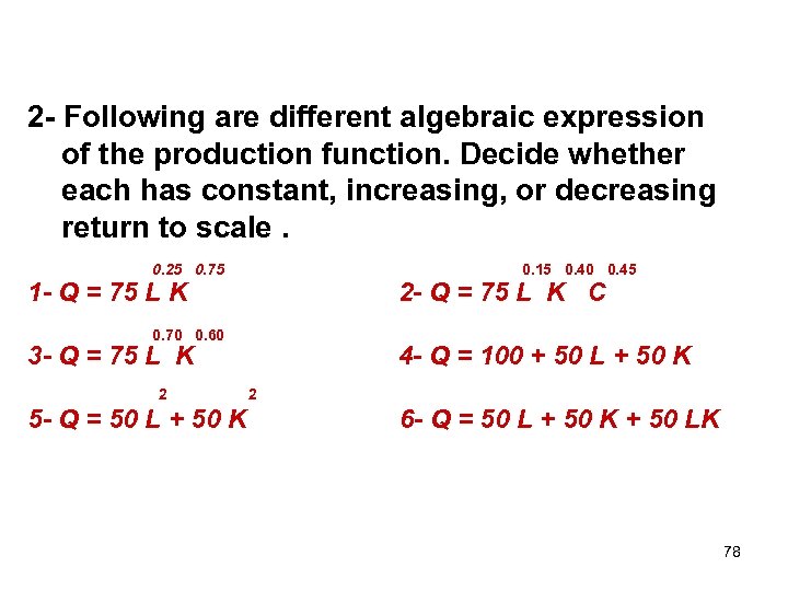
2 - Following are different algebraic expression of the production function. Decide whether each has constant, increasing, or decreasing return to scale. 0. 25 0. 75 0. 15 0. 40 0. 45 1 - Q = 75 L K 2 - Q = 75 L K C 0. 70 0. 60 3 - Q = 75 L K 2 5 - Q = 50 L + 50 K 4 - Q = 100 + 50 L + 50 K 2 6 - Q = 50 L + 50 K + 50 LK 78

3 - The owner of a car wash is trying to decide on the number of people to employ based on the following short production function: Q = 6 L – 0. 5 L² Where Q = No. of car washes per hour L = No. of workers a- Generate a schedule showing TP, AP, MP. , then graph it. b- Suppose the price for a basic car wash (no under coating , no wax treatments etc. ) in his area of business is LE 5. How many people should he hireif he pays each worker LE 6 / he. ? c- Suppose he consider hiring students on a part time basis for LE 4 hr. . Do you think he should hire more students at this lower rate ? Explain. 79

Part (6) : Theory & Estimation of Cost Why should firms incur costs? Why do they exist? The existence of costs of production is attributable directly to the existence of scarcity. 1 - Cost Concepts a- Implicit Costs. We shall refer to nonpecuniary costs as implicit costs , economists identify it as opportunity costs. b- Explicit Costs. is pecuniary, accounting cost by virtue of the fact that such money-denominated costs are visible, readily monitored, and hence easily included by accountants 80

Accounting Costs Subdivided into two categories: - Disbursement Costs. Disbursement costs are those out of pocket money payments from the enterprise to parties who provide services or resources to the enterprise. such as the payroll, payments for energy, the raw materials, etc. - Non-disbursement cost: depreciation (capital consumption). is an allowance for the decline in the value of the capital stock which is attributable to the using-up of part of the enterprise's capital equipment during the production (the accounting) period. An allowance for depreciation is not paid out (disbursed) to any party outside the enterprise; rather it is in a sense paid to the enterprise itself for the use of the capital equipment owned by the enterprise. 81

Spill-Over Costs: A final example of costs which are irrelevant to current decision making consists of social or spill-over costs. i. e. , the negative aspects of production which descend upon members of society other than the production decision maker? For example, air, water, and noise pollution are the unfortunate by-products of production processes which affect parties outside the enterprise. These spill-over costs, however, are irrelevant to the production decision context unless or until either the production decision maker experiences a twinge of conscience, or the authorities require the firm to prevent, clean-up, or compensate those who have been harmed. We may say, then, that while such spill-over costs currently are irrelevant to the production decision context, they always have the potential for becoming relevant costs and should not be ignored entirely by the production decision maker. 82

Variable and Fixed Costs 1 - Variable costs (VC): are those which vary with the level of productive output. Variable costs are always relevant to the rate-of-production decision. 2 - Fixed or overhead costs: are associated with the existence of the manager, the plant, and the equipment. Such as contractual salaries and insurance premiums. They continue at the same levels or rates irrespective of the rate of production, even if it is zero. Once the plant has been put in place, these fixed or overhead costs are, "sunk" costs, and sunk costs are not relevant to any rate-of-production decisions 83

Accounting profit and economic profit Accounting profit is the explicit, money-denominated revenues realized by the enterprise during an accounting period, less the explicit, money-denominated costs which are incurred in that same period. Accounting profit does not include any implicit costs, . the computation of an enterprise's accounting profit may over- or understate its true (economic) profit and thereby lead to erroneous decisions. Economic profit is the result of the economist's effort to recognize all benefits (implicit as well as money revenues) and costs (opportunity costs as well as accounting costs) accruing to the enterprise. Economic costs are all of the costs which are relevant to decision making, whether or not money disbursements were made and whether or not they are recognized in formal accounting A critical distinction between a "good management" and "poor management" may lie in the ability of the decision maker to recognize the implicit costs and benefits of managerial decisions. 84

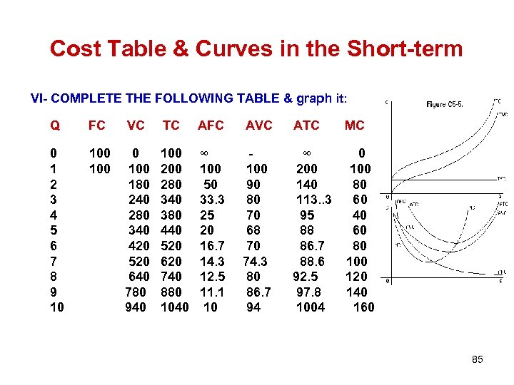
Cost Table & Curves in the Short-term VI- COMPLETE THE FOLLOWING TABLE & graph it: Q FC VC TC AFC AVC ATC MC 0 1 2 3 4 5 6 7 8 9 10 100 180 240 280 340 420 520 640 780 940 100 280 340 380 440 520 620 740 880 1040 ∞ 100 50 33. 3 25 20 16. 7 14. 3 12. 5 11. 1 10 100 90 80 70 68 70 74. 3 80 86. 7 94 ∞ 200 140 113. . 3 95 88 86. 7 88. 6 92. 5 97. 8 1004 = ∆ TC/ ∆Q 0 100 80 60 40 60 80 100 120 140 160 85

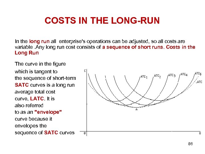
COSTS IN THE LONG-RUN In the long run all enterprise's operations can be adjusted, so all costs are variable. Any long run cost consists of a sequence of short runs. Costs in the Long Run The curve in the figure which is tangent to the sequence of short-term SATC curves is a long run average total cost curve, LATC. It is also referred to as an "envelope" curve because it envelopes the sequence of SATC curves 86

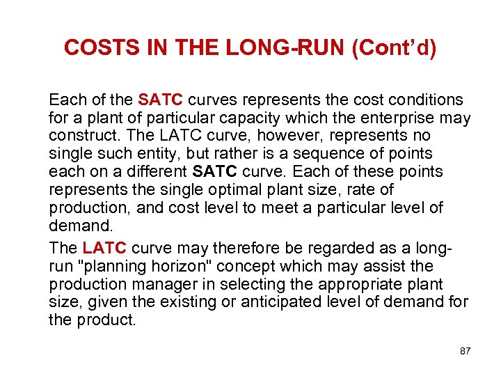
COSTS IN THE LONG-RUN (Cont’d) Each of the SATC curves represents the cost conditions for a plant of particular capacity which the enterprise may construct. The LATC curve, however, represents no single such entity, but rather is a sequence of points each on a different SATC curve. Each of these points represents the single optimal plant size, rate of production, and cost level to meet a particular level of demand. The LATC curve may therefore be regarded as a longrun "planning horizon" concept which may assist the production manager in selecting the appropriate plant size, given the existing or anticipated level of demand for the product. 87

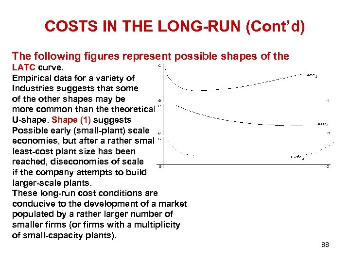
COSTS IN THE LONG-RUN (Cont’d) The following figures represent possible shapes of the LATC curve. Empirical data for a variety of Industries suggests that some of the other shapes may be more common than theoretical U-shape. Shape (1) suggests Possible early (small-plant) scale economies, but after a rather small least-cost plant size has been reached, diseconomies of scale if the company attempts to build larger-scale plants. These long-run cost conditions are conducive to the development of a market populated by a rather larger number of smaller firms (or firms with a multiplicity of small-capacity plants). 88

COSTS IN THE LONG-RUN (Cont’d) Shape(2) depicts long-run cost conditions characterized by the progressive, though gradual, exploitation of economies of scale which never seem to reach exhaustion. A market characterized by these long Run cost conditions will tend to be populated by a rather smaller number of larger-sized firms, and perhaps ever fewer firms as time passes and competition ensues. Economists classify such a market as oligopolistic. The ultimate end of competitive evolution in such a market might be a single, very large surviving firm, a so-called "natural monopoly. " Shape(3) may have involved a few minor scale economies as firms grew from very small size at start-up, and could eventually reach a range of diseconomies of large scale if existing firms Grow much larger. But the salient characteristic of LATC curve is that it is flat-bottomed, i. e. , there are no significant scale economies to be exploited or diseconomies to be suffered over a very wide range of plant sizes. . 89

Mathematical Specification and Empirical Estimation of Cost Functions TC = b 0 + b 1 Q + b 2 Q 2 + b 3 Q 3, from which may be derived MC = d. TC/d. Q = b 1 + 2 b 2 Q + 3 b 3 Q 2 and ATC = TC/Q = b 0/Q + b 1 + b 2 Q + b 3 Q 2. If b 3 turns out not to be statistically significant but both b 1 and b 2 are significant, the model may be respecified as a quadratic of form TC = b 0 + b 1 Q + b 2 Q 2, from which may be derived MC = d. TC/d. Q = b 1 + 2 b 2 Q and ATC = TC/Q = b 0/Q + b 1 + b 2 Q. if upon regression analysis of the quadratic form the coefficient b 2 appears not to be statistically significant, the equation may be respecified as a linear form, TC = b 0 + b 1 Q, from which may be derived MC = d. TC/d. Q = b 1, and ATC = TC/Q = b 0/Q + b 1. 90

cost-function simulation model The Management of Costs Whether the management of the firm develops cost-function simulation model or not, the cost related job involves many facets: (1) in the long run, selecting the most efficient technology for producing the selected products; (2) with that technology, selecting the scale of plant with an output range which is most compatible with current and expected future levels of demand for the products; (3) given the right scale of plant, selecting the appropriate output level to meet the enterprise's goals (profit aximization, cost minimization, etc. ); (4) for the target level of output, selecting the appropriate internal allocation of the enterprise's resources, i. e. , the most efficient combination of inputs, given the available input prices; (5) operating efficiently and without waste, i. e. , to operate at points on the enterprise's production function surface (not below it) and on its respective cost curve (not above it). Furthermore, economists can argue that if the goal of the enterprise is to maximize profits, and if it does so operate to maximize profits without monopolizing its markets or exploiting its resources, it will also meet a desirable social objective of efficiency in the allocation of resources. 91

Perfect Competition The descriptive characteristics: (1) There is a large number of very small firms which operate within the same product market. (2) The single product which they produce and market is essentially homogeneous across the member firms. (3) The member firms have virtually identical managerial capacities; they use essentially the same technologies; no one of them has or can acquire any special expertise which is not available to all of the others. (4) All participants in the market have access to the same information about changing market conditions Consequences and behavioral patterns for firms in the purely competitive market : 92

Perfect Competition (Cont’d) ( a) Entry into the market is easy; entry may be accomplished quickly because of the ready availability of common technology, and with very little capital investment. (b) Exit from the market is likewise easy, i. e. , the firm can dispose of its capital assets quickly and with very little loss of value. (c) Once a decision has been made to enter the competitive market there is likely be very little incentive or effort to exercise further entrepreneurship, except the decision to exit the market. (d) The atomistic size and limited financial resources of the competitive firm militate against its acquisition of any special managerial or technical expertise; firms are unable successfully to differentiate their products, and no firm can attain any position of market dominance. 93

Perfect Competition (Cont’d) (e) Because of the common knowledge of changing market conditions, all participants in the market become aware of such changes simultaneously, and all adjust at approximately the same rates. (f) Because of the large number and atomistic size of sellers, competition is essentially anonymous; no seller is aware of or concerned about the identities of other sellers. (g) A common price likely emerges in the market, and no market participant finds incentive to try to charge any price higher or lower than the market price. (h) Due to the absence of successful product differentiation, there is little or no point in advertising the firm's product characteristics or its price. (i) Supernormal and subnormal profits in the competitive market, although they may occur, are fleeting; profits tend toward the economically normal level of opportunity cost (what the firm can realize in the next best alternative application of its resources). 94

A Firm in a Purely Competitive Industry The general principle that govern output decision making when the goal is to maximize profit is to: P(MR) =MC increase Q if MR > MC, but to decrease Q if , MR < MC. MR is easy to identify in the purely competitive market because it is equal to price, and the MR curve is coincident with the demand curve. However, MC is not directly observable. It can be computed for any output level if the equation of the TC or MC curve is known, but knowing either of these equations probably required a costly data collection and model specification and estimation process. Incremental cost can be computed more cheaply from data for two different output levels, but it is only an approximation to true marginal cost 95

The Operate vs. Shut-Down Criterion in the Short Run It may be rational to shut-down operations in the short-run if the revenue generated by selling the output cannot cover even the operating costs (or variable costs) of producing the output. Assuming cubic production and cost functions, the shut-down criterion can be illustrated in the above figure at any Qt for which AR (P) < AVC, In these circumstances, the firm should not operate because the revenue resulting from operation would not cover all of the operating costs, and could make no contribution at all to the overhead costs. In shut-down mode, the firm minimizes its losses by incurring only the fixed costs. The fixed costs, which continue in the short run whether the firm operates or not, can be saved (or avoided) only by exiting the industry. . 96

Operate vs. Shut-Down Criterion in the Short Run I-You have given the following cost function: TC = 100 + 600 Q – 3 Q² + 0. 1 Q³ TC = 100 + 600 Q – 3 Q² TC = 100 + 600 Q 1 - compute the AVC, AC, and MC for each function. Plot them in graph. 2 - In each case , indicate the point at which diminishing returns occur, also indicate the point of max. cost efficiency. 3 - For each function, discuss the relationship b/w MC, AVC , and b/w MC and AC, and the relationship b/w AVC and AC. II-The demand cost function for a company are estimated to be as follows: p = 170 – 5 Q TC = 50 + 80 Q – 10 Q 2 + 0. 6 Q 3 97

Operate vs. Shut-Down Criterion in the Short Run a. What price should the company charge if it wishes to maximize its profits in the short run. b. What price should it charge if it wishes to maximize its revenue in the short run? c. suppose the company lacks confidence in the accuracy of cost estimates expressed in a cubic equation and simply wants to use a linear approximation. Suggest a linear representation of this cubic equation. What difference would it make on the recommended profit maximizing and revenue maximizing prices? 98

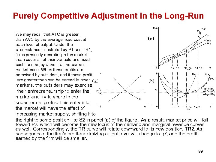
Purely Competitive Adjustment in the Long-Run We may recall that ATC is greater than AVC by the average fixed cost at each level of output. Under the circumstances illustrated by P 1 and TR 1, firms presently operating in the market t can cover all of their variable and fixed costs and enjoy a profit at the current market price. When these profits are perceived by outsiders, and if these profits are greater than can be earned in other markets, the outsiders may exercise their entrepreneurship to enter the market and try to share in the supernormal profits. This entry into the market will have the effect of increasing market supply, shifting it to the right to some position like S 2 in panel (a) of the figure. As a result, market price will fall toward P 2, which will become the new locus of the demand marginal revenue curves as well. Correspondingly, the TR curve will rotate downward to its new position, TR 2. As consequence, the firm's profit-maximizing output level will change to q 7, and the profit earned by the firm will be smaller. 99

Purely Competitive Adjustment in the Long-Run driven by continuing entry into the market, could continue until the price falls to P 2 and the total revenue curve rotates to position TR 2; here, supernormal profits are eliminated and the market price just covers the firm's variable and fixed costs, allowing only a normal return to the firm's ownership interest. The important point is that with no effective way for firms to prevent entry into the market, all super-normal profits will be competed away. But no firm in the market will be suffering because each will be paying or earning normal returns for all of the resources under its employ. Capital and entrepreneurship, having entered the market, will continue in their present occupation until the prospect of supernormal profits appears elsewhere. 100

Purely Competitive Adjustment in the Long-Run Managers who committed to plants like ATCm or ATC 1 may find their firms realizing losses relative to firms whose managers chose to build a least-cost plant. They are stuck with plants which are too small or too large for the duration of the lives of the plant and equipment. Their short-run options are to continue to operate while suffering losses if Pe happens to exceed their average variable cost, or to shut-down if Pe is less than their average variable cost. If price remains as low as Pe, the firms which are realizing losses have the option of exiting the market. Exit from the market will likely involve capital losses if the plant and equipment cannot be economically converted to other applications, or if they must be sold at prices below their depreciated book values. 101

2 -Your are given the following LTC function: TC = 160 Q- 20 Q² + 1. 2 Q³ a- Calculate the LATC & the LMC. Graph these cost. b- Describe the nature of of this function’s scale economies. Over what range of output does economies of scale exist? Diseconomies of scale ? Show this in the graph. 3 - The demand cost function for a company are estimated to be as follows: P = 100 – 8 Q TC = 50 + 80 Q – 10 Q² + o. 6 Q³ a- What quantity and price should the company charge if it wishes to maximize its profit in the short-run ? Calculate the max. profit. b- What quantity and price should it charge if wishes to maximize its revenue in the short-run ? c- Suppose the company lacks confidence in the accuracy of cost estimates expressed in a cubic equation and simply wants to use a linear approximation. Suggest a linear representation of the cubic equation. What difference would it make on the recommended profit maximizing and revenue-maximizing prices 102

The following represents (D) & (D): in a perfectly competitive market. D = 3000 – 10 P S = - 1000 + 10 P a- At what P would D = 0 b- At what P would S = 0 , c- Graph both D & S d- What are the Qe & Pe ? Suppose the industry (S) consist of 100 identical firms, Determine The Q that should be produced by each individual firm. e- Suppose that the commodity is a normal good & average income increased and moved D upward to the right, changing the D equation to: D 1 = 3500 - 10 P. , what is the effect on Qe & Pe? Determine The Q that should be produced by each individual firm. f- Suppose another 50 new firms enter the market due to the increase in D, so the new S is : S 2 = -500 + 10 P, What are the new Qe & Pe ? Determine The Q that should be produced by each individual firms. g- Show these changes on the graph 103

Assume the following is the production function for each of the 150 identical firms : 0. 5 Q = 100 K L 104

Final Exam I- Write Short Notes on 4/6 II- Three Problems 2/3 Slide 64 , 79 and 80 , 85 105