Cost Risk Allocation Objectives Tendencies and Limitations John

Cost Risk Allocation Objectives, Tendencies and Limitations John Sandberg Master Programmer, ACEIT Joint ISPA/SCEA Conference, June 12 -15, 2007 Los Angeles Albuquerque 7 April 2007 Colorado Springs Charleston Cleveland Washington, D. C. Boston Columbus Ft. Meade Denver New Orleans Chantilly Ft. Monmouth Oklahoma City Huntsville Montgomery Silver Spring Dayton Ogden Santa Barbara Patuxent River Warner Robins AFB Pensacola San Diego Vandenberg AFB 1

Overview n Overview 2 -3 minutes Proverb n What Is Cost Risk Allocation? Knowledge is better than blind practice. 10 -15 minutes n Defining The Threat -Fortune Cookie 10 -15 minutes n Minimizing Average Budget Overrun Lucky numbers: 7 9 23 36 41, 19 15 -20 minutes n Minimizing Budget Overrun Semi-Variance 20 -30 minutes n In Conclusion 2 -3 minutes 27 April 2007 Copyright (c) 2007 by Tecolote Research, Inc. 2

What Is Cost Risk Allocation? 27 April 2007 Copyright (c) 2007 by Tecolote Research,

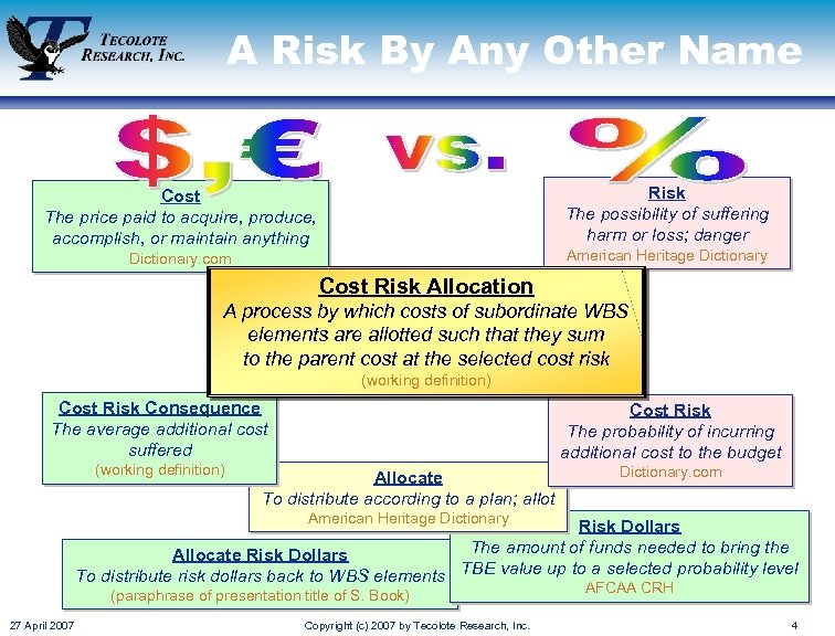
A Risk By Any Other Name Risk The possibility of suffering harm or loss; danger Cost The price paid to acquire, produce, accomplish, or maintain anything American Heritage Dictionary. com Cost Risk Allocation A process by which costs of subordinate WBS elements are allotted such that they sum to the parent cost at the selected cost risk (working definition) Cost Risk Consequence The average additional cost suffered (working definition) Cost Risk The probability of incurring additional cost to the budget Allocate To distribute according to a plan; allot Dictionary. com American Heritage Dictionary Risk Dollars The amount of funds needed to bring the Allocate Risk Dollars To distribute risk dollars back to WBS elements TBE value up to a selected probability level (paraphrase of presentation title of S. Book) 27 April 2007 Copyright (c) 2007 by Tecolote Research, Inc. AFCAA CRH 4

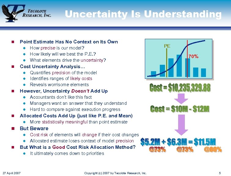
Uncertainty Is Understanding n Point Estimate Has No Context on Its Own How precise is our model? l How likely will we beat the P. E. ? l What elements drive the uncertainty? l n PE 70% Cost Uncertainty Analysis… Quantifies precision of the model l Identifies ranges of likely costs l Reveals worrisome elements l n However, Uncertainty Doesn’t Add Up Accountants don’t like this fact l Managers want an answer that they understand l Hard to compare against execution progress l n Allocated Costs Add Up (just like P. E. and Mean) l n More statistically meaningful than point estimate But Beware Cost risk of elements will change if their cost changes l Allocated estimate loses context of model precision l n But What is a Good Cost Risk Allocation Method? l 27 April 2007 It ultimately comes down to priorities Copyright (c) 2007 by Tecolote Research, Inc. 5

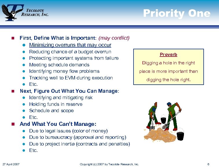
Priority One n First, Define What is Important: (may conflict) l Minimizing overruns that may occur l l l n Reducing chance of a budget overrun Protecting important systems from failure Meeting schedule demands Identifying money flow problems Tracking well to EVM during execution Etc. Proverb Digging a hole in the right place is more important than digging the hole right. Next, Figure Out What You Can Manage: Identifying and mitigating risk l Holding funds in reserve l Schedule and scope l Etc. l n And What You Can’t Manage: l Due to legal issues (color of money) l Due to bureaucracy (approval and reporting) l Due to project inertia (contracts and penalties) l Etc. 27 April 2007 Copyright (c) 2007 by Tecolote Research, Inc. 6

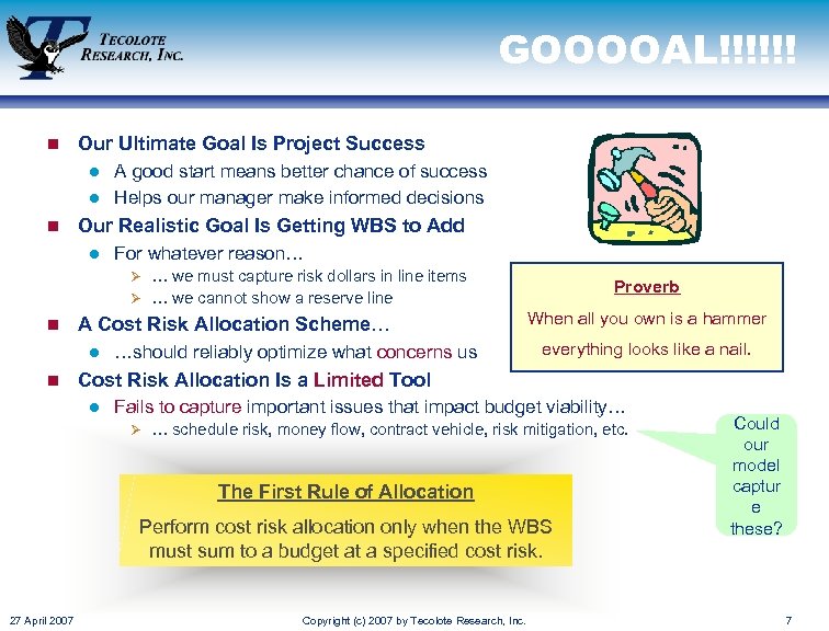
GOOOOAL!!!!!! n Our Ultimate Goal Is Project Success A good start means better chance of success l Helps our manager make informed decisions l n Our Realistic Goal Is Getting WBS to Add l For whatever reason… … we must capture risk dollars in line items Ø … we cannot show a reserve line Ø n A Cost Risk Allocation Scheme… l n …should reliably optimize what concerns us Proverb When all you own is a hammer everything looks like a nail. Cost Risk Allocation Is a Limited Tool l Fails to capture important issues that impact budget viability… Ø … schedule risk, money flow, contract vehicle, risk mitigation, etc. The First Rule of Allocation Perform cost risk allocation only when the WBS must sum to a budget at a specified cost risk. 27 April 2007 Copyright (c) 2007 by Tecolote Research, Inc. Could our model captur e these? 7

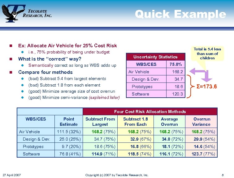
Quick Example n Ex: Allocate Air Vehicle for 25% Cost Risk l n Uncertainty Statistics What is the “correct” way? l n i. e. , 75% probability of being under budget Semantically correct as long as WBS adds up l l l 75. 0% Air Vehicle Compare four methods l WBS/CES (bad) Subtract 5. 4 from largest elements (bad) Subtract 1. 8 from each element (good) Minimize average size of cost overrun (good) Minimize semi-variance (explained later) Total is 5. 4 less than sum of children 168. 2 Design & Dev. 34. 7 Prototypes 18. 6 Software Σ=173. 6 120. 3 Four Cost Risk Allocation Methods WBS/CES Air Vehicle Design & Dev. Prototypes Software 27 April 2007 Point Estimate Subtract From Largest Subtract 1. 8 From Each Average Overrun Variance 111. 5 (32%) 168. 2 (75%) 25. 0 (25%) 34. 7 (75%) 32. 9 (67%) 34. 0 (72%) 29. 9 (54%) 9. 7 (20%) 18. 6 (75%) 16. 8 (66%) 18. 1 (72%) 14. 6 (54%) 76. 8 (41%) 114. 9 (71%) 118. 5 (74%) 116. 1 (72%) 123. 7 (77%) Copyright (c) 2007 by Tecolote Research, Inc. 8

Defining The Threat 27 April 2007 Copyright (c) 2007 by Tecolote Research, Inc. 9

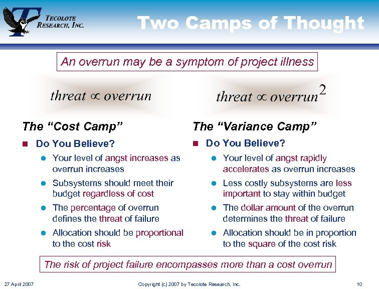
Two Camps of Thought An overrun may be a symptom of project illness The “Cost Camp” The “Variance Camp” n Do You Believe? l Your level of angst increases as overrun increases l Your level of angst rapidly accelerates as overrun increases l Subsystems should meet their budget regardless of cost l Less costly subsystems are less important to stay within budget l The percentage of overrun defines the threat of failure l The dollar amount of the overrun determines the threat of failure l Allocation should be proportional to the cost risk l Allocation should be in proportion to the square of the cost risk The risk of project failure encompasses more than a cost overrun 27 April 2007 Copyright (c) 2007 by Tecolote Research, Inc. 10

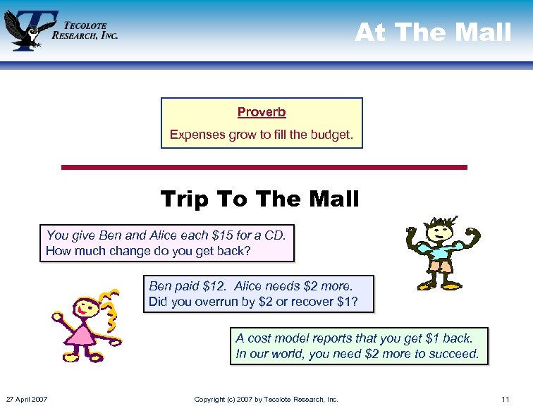
At The Mall Proverb Expenses grow to fill the budget. Trip To The Mall You give Ben and Alice each $15 for a CD. How much change do you get back? Ben paid $12. Alice needs $2 more. Did you overrun by $2 or recover $1? A cost model reports that you get $1 back. In our world, you need $2 more to succeed. 27 April 2007 Copyright (c) 2007 by Tecolote Research, Inc. 11

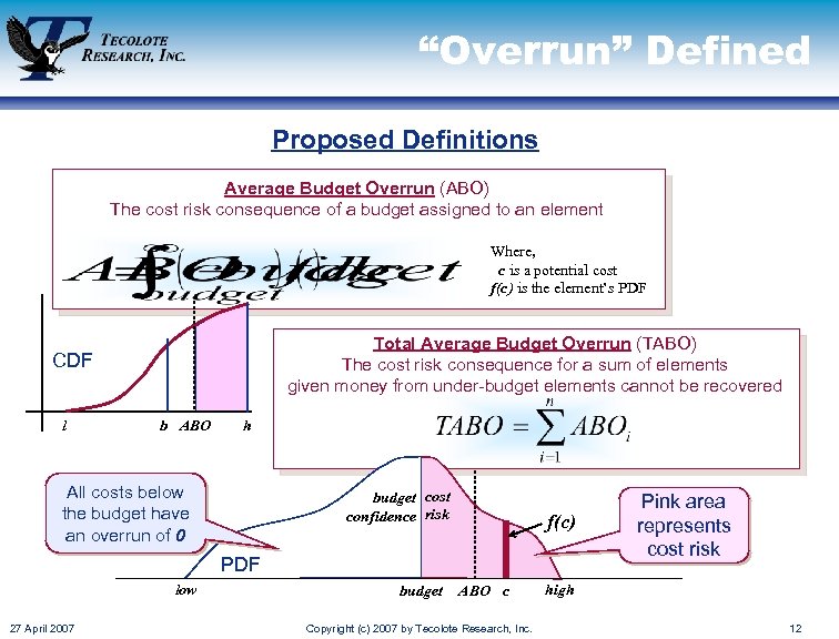
“Overrun” Defined Proposed Definitions Average Budget Overrun (ABO) The cost risk consequence of a budget assigned to an element Where, c is a potential cost f(c) is the element’s PDF Total Average Budget Overrun (TABO) The cost risk consequence for a sum of elements given money from under-budget elements cannot be recovered CDF l b ABO h All costs below the budget have an overrun of 0 budget cost confidence risk f(c) PDF low 27 April 2007 budget ABO c Copyright (c) 2007 by Tecolote Research, Inc. Pink area represents cost risk high 12

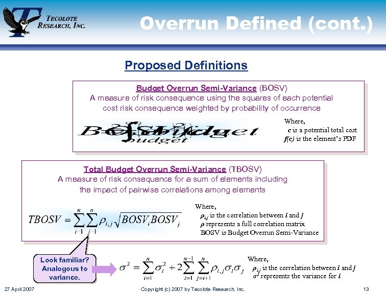
Overrun Defined (cont. ) Proposed Definitions Budget Overrun Semi-Variance (BOSV) A measure of risk consequence using the squares of each potential cost risk consequence weighted by probability of occurrence Where, c is a potential total cost f(c) is the element’s PDF Total Budget Overrun Semi-Variance (TBOSV) A measure of risk consequence for a sum of elements including the impact of pairwise correlations among elements Where, ρi, j is the correlation between i and j ρ represents a full correlation matrix BOSV is Budget Overrun Semi-Variance Where, ρi, j is the correlation between i and j σ2 represents the variance for i Look familiar? Analogous to variance. 27 April 2007 Copyright (c) 2007 by Tecolote Research, Inc. 13

Minimizing Average Cost Overrun 27 April 2007 Copyright (c) 2007 by Tecolote Research, Inc.

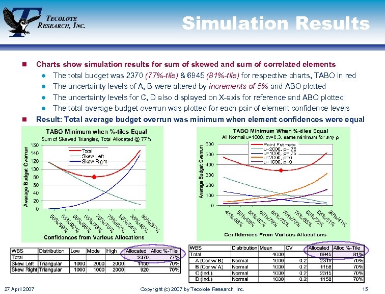
Simulation Results n n 27 April 2007 Charts show simulation results for sum of skewed and sum of correlated elements l The total budget was 2370 (77%-tile) & 6945 (81%-tile) for respective charts, TABO in red l The uncertainty levels of A, B were altered by increments of 5% and ABO plotted l The uncertainty levels for C, D also displayed on X-axis for reference and ABO plotted l The total average budget overrun was plotted for each pair of element confidence levels Result: Total average budget overrun was minimum when element confidences were equal Copyright (c) 2007 by Tecolote Research, Inc. 15

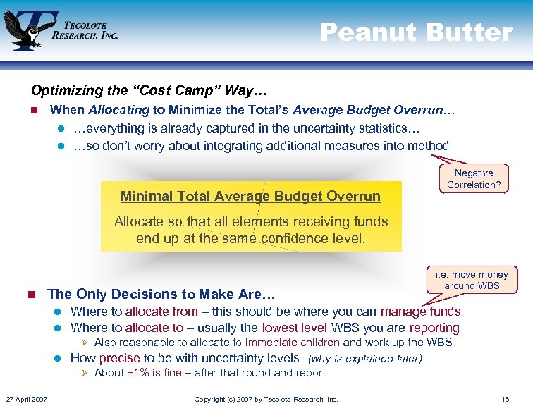
Peanut Butter Optimizing the “Cost Camp” Way… n When Allocating to Minimize the Total’s Average Budget Overrun… l …everything is already captured in the uncertainty statistics… l …so don’t worry about integrating additional measures into method Minimal Total Average Budget Overrun Negative Correlation? Allocate so that all elements receiving funds end up at the same confidence level. i. e. move money around WBS n The Only Decisions to Make Are… l Where to allocate from – this should be where you can manage funds l Where to allocate to – usually the lowest level WBS you are reporting Also reasonable to allocate to immediate children and work up the WBS l How precise to be with uncertainty levels (why is explained later) Ø About ± 1% is fine – after that round and report Ø 27 April 2007 Copyright (c) 2007 by Tecolote Research, Inc. 16

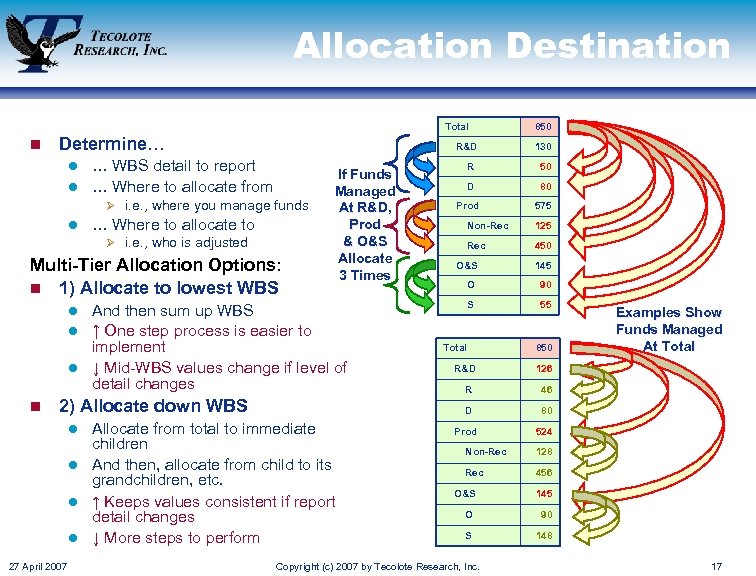
Allocation Destination Total n Determine… R&D … WBS detail to report l … Where to allocate from l Ø i. e. , where you manage funds l … Where to allocate to Ø i. e. , who is adjusted Multi-Tier Allocation Options: n 1) Allocate to lowest WBS If Funds Managed At R&D, Prod & O&S Allocate 3 Times And then sum up WBS l ↑ One step process is easier to implement l ↓ Mid-WBS values change if level of detail changes Allocate from total to immediate children l And then, allocate from child to its grandchildren, etc. l ↑ Keeps values consistent if report detail changes l ↓ More steps to perform 27 April 2007 50 D 80 Prod 575 Non-Rec 125 Rec 450 O&S 145 O 90 S 55 Total R&D 850 Examples Show Funds Managed At Total 126 R 46 D 2) Allocate down WBS l 130 R l n 850 80 Prod 524 Non-Rec 128 Rec 456 O&S 145 O 90 S 148 Copyright (c) 2007 by Tecolote Research, Inc. 17

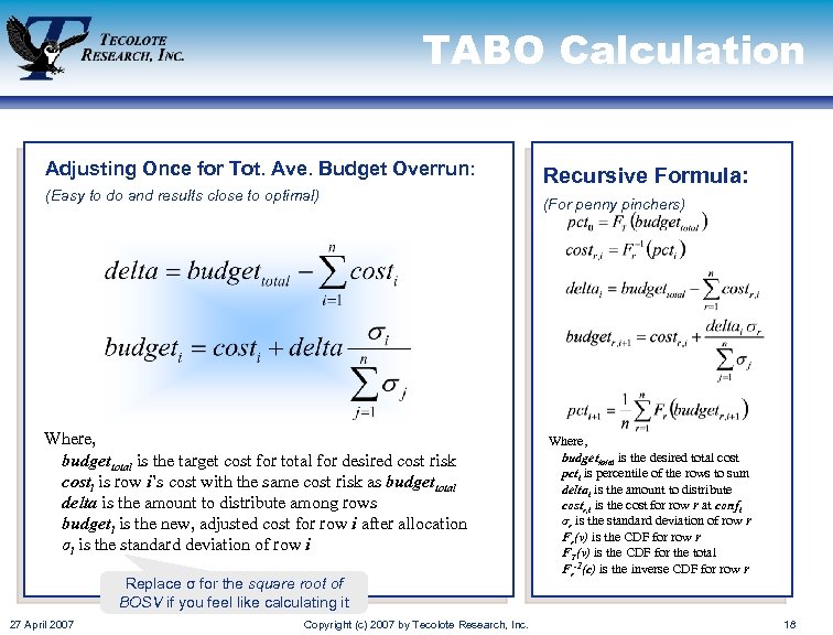
TABO Calculation Adjusting Once for Tot. Ave. Budget Overrun: (Easy to do and results close to optimal) Where, budgettotal is the target cost for total for desired cost risk costi is row i’s cost with the same cost risk as budgettotal delta is the amount to distribute among rows budgeti is the new, adjusted cost for row i after allocation σi is the standard deviation of row i Replace σ for the square root of BOSV if you feel like calculating it 27 April 2007 Copyright (c) 2007 by Tecolote Research, Inc. Recursive Formula: (For penny pinchers) Where, budgettotal is the desired total cost pcti is percentile of the rows to sum deltai is the amount to distribute costr, i is the cost for row r at confi σr is the standard deviation of row r Fr(v) is the CDF for row r FT(v) is the CDF for the total Fr-1(c) is the inverse CDF for row r 18

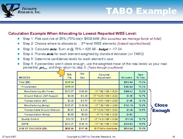
TABO Example Calculation Example When Allocating to Lowest Reported WBS Level: l l l Step 1: Pick cost risk of 25% (75%-tile)= $608. 94 M (this assumes we manage funds at total) Step 2: Choose where to allocate to… 3 rd level WBS elements (lowest reported level) Step 3: Calculate delta: Sum at @ 75% = 625. 98 - budget = -17. 04 Step 4: Prorate delta for each element weighted by standard deviation (or TABO) Step 5: Determine confidence levels for each element’s cost Step 6: If percentiles aren’t close enough, use the weighted mean of the new levels as your next percentile, pcti+1, and then return to step 3. (Twice through is sufficient) WBS/CES 75% -Tile Total ($M) Procurement Manufacturing (Air Force) Std Allocated New %-Tiles $608. 94 75. 0% $385. 66 $393. 92 75. 2% Dev Calculate Adjustment $272. 67 $ 68. 80 -17 * 69 / 188 = -6. 24 $266. 43 72. 2% Ground Station LRIP Support $0. 88 $ 0. 25 -17 * 0. 25 / 188 = -0. 02 $0. 86 72. 7% Transportation (AF) $2. 00 $ 0. 57 -17 * 0. 57 / 188 = -0. 05 $1. 95 72. 7% $125. 87 $ 29. 59 -17 * 29 / 188 = -2. 68 $123. 19 72. 2% Transportable Ground Stations $0. 91 $ 0. 24 -17 * 0. 24 / 188 = -0. 02 $0. 89 72. 5% Transportation (Army) $0. 60 $0. 00 -17 * 0 / 188 = -0. 00 $0. 60 $10. 78 $ 4. 27 -17 * 4. 3 / 188 = -0. 39 $10. 39 72. 7% $212. 27 $ 84. 14 -17 * 84 / 188 = -7. 64 $204. 63 72. 5% $625. 98 $187. 86 $-17. 04 to distribute $608. 94 75. 0% Manufacturing (Army) Quality Control SEPM SUM OF CHILDREN ($M) 27 April 2007 Copyright (c) 2007 by Tecolote Research, Inc. Close Enough 19

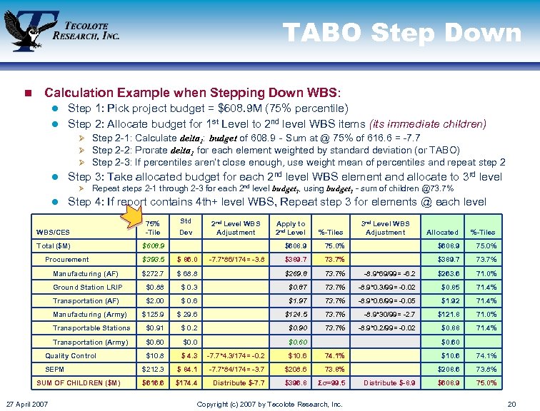
TABO Step Down n Calculation Example when Stepping Down WBS: Step 1: Pick project budget = $608. 9 M (75% percentile) l Step 2: Allocate budget for 1 st Level to 2 nd level WBS items (its immediate children) Ø Step 2 -1: Calculate delta 1: budget of 608. 9 - Sum at @ 75% of 616. 6 = -7. 7 l Ø Step 2 -2: Prorate delta 1 for each element weighted by standard deviation (or TABO) Ø Step 2 -3: If percentiles aren’t close enough, use weight mean of percentiles and repeat step 2 l Step 3: Take allocated budget for each 2 nd level WBS element and allocate to 3 rd level Ø l Repeat steps 2 -1 through 2 -3 for each 2 nd level budget 2, using budget 2 - sum of children @73. 7% Step 4: If report contains 4 th+ level WBS, Repeat step 3 for elements @ each level WBS/CES 75% -Tile Total ($M) Std $608. 9 Procurement 2 nd Level WBS Adjustment 3 nd Level WBS Adjustment Allocated %-Tiles 75. 0% $608. 9 75. 0% $389. 7 73. 7% $393. 5 $ 86. 0 $272. 7 $ 68. 8 $269. 8 73. 7% -8. 9*69/99= -6. 2 $263. 6 71. 0% Ground Station LRIP $0. 88 $ 0. 3 $0. 87 73. 7% -8. 9*0. 3/99= -0. 02 $0. 85 71. 4% Transportation (AF) $2. 00 $ 0. 6 $1. 97 73. 7% -8. 9*0. 6/99= -0. 05 $1. 92 71. 4% Manufacturing (Army) $125. 9 $ 29. 6 $124. 5 73. 7% -8. 9*30/99= -2. 7 $121. 8 71. 0% Transportable Stations $0. 91 $ 0. 2 $0. 90 73. 7% -8. 9*0. 2/99= -0. 02 $0. 88 71. 4% Transportation (Army) $0. 60 $10. 8 $ 4. 3 -7. 7*4. 3/174= -0. 2 $10. 6 74. 1% $212. 3 $ 84. 1 -7. 7*84/174= -3. 7 $208. 6 73. 8% $616. 6 $174. 4 Distribute $-7. 7 $396. 8 Σσ=99. 5 $608. 9 75. 0% Manufacturing (AF) Quality Control SEPM SUM OF CHILDREN ($M) 27 April 2007 -7. 7*86/174= -3. 8 %-Tiles $608. 9 Dev Apply to 2 nd Level $0. 60 Copyright (c) 2007 by Tecolote Research, Inc. Distribute $-8. 9 20

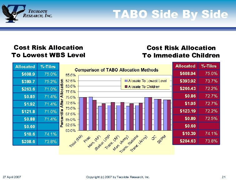
TABO Side By Side Cost Risk Allocation To Lowest WBS Level Cost Risk Allocation To Immediate Children Allocated %-Tiles $608. 9 75. 0% $608. 94 75. 0% $389. 7 75. 2% $393. 92 73. 7% $263. 6 71. 0% $266. 43 72. 2% $0. 85 71. 4% $0. 86 72. 7% $1. 92 71. 4% $1. 95 72. 7% $121. 8 71. 0% $123. 19 72. 2% $0. 88 71. 4% $0. 89 72. 5% $0. 60 $10. 6 $10. 39 74. 1% $208. 6 27 April 2007 74. 1% 73. 8% $204. 63 73. 8% Copyright (c) 2007 by Tecolote Research, Inc. 21

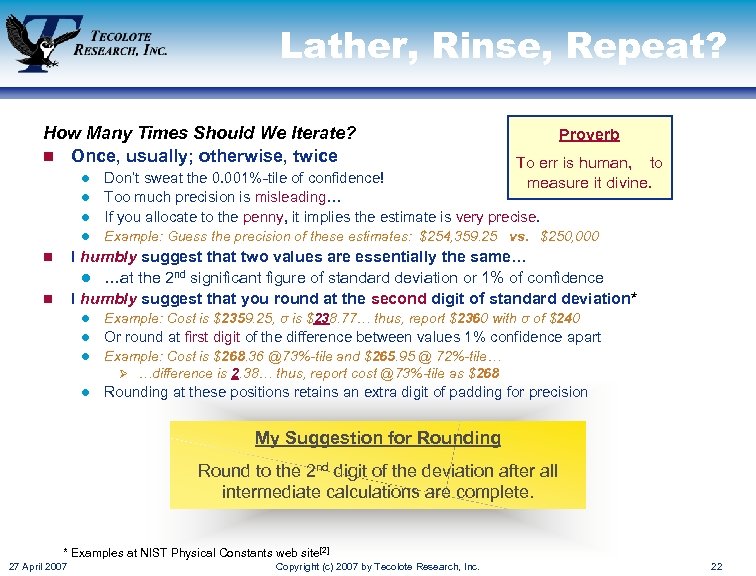
Lather, Rinse, Repeat? How Many Times Should We Iterate? n Once, usually; otherwise, twice Proverb To err is human, to Don’t sweat the 0. 001%-tile of confidence! measure it divine. l Too much precision is misleading… l If you allocate to the penny, it implies the estimate is very precise. l l Example: Guess the precision of these estimates: $254, 359. 25 vs. $250, 000 I humbly suggest that two values are essentially the same… l …at the 2 nd significant figure of standard deviation or 1% of confidence I humbly suggest that you round at the second digit of standard deviation* n n l Example: Cost is $2359. 25, σ is $238. 77… thus, report $2360 with σ of $240 l Or round at first digit of the difference between values 1% confidence apart l Example: Cost is $268. 36 @73%-tile and $265. 95 @ 72%-tile… Ø …difference is 2. 38… thus, report cost @73%-tile as $268 l Rounding at these positions retains an extra digit of padding for precision My Suggestion for Rounding Round to the 2 nd digit of the deviation after all intermediate calculations are complete. * Examples at NIST Physical Constants web site[2] 27 April 2007 Copyright (c) 2007 by Tecolote Research, Inc. 22

Minimizing Overrun Semi-Variance 27 April 2007 Copyright (c) 2007 by Tecolote Research, Inc. 23

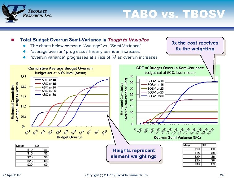
TABO vs. TBOSV n Total Budget Overrun Semi-Variance Is Tough to Visualize l l l The charts below compare “Average” vs. “Semi-Variance” “average overrun” progresses linearly as mean increases “overrun variance” progresses at a rate of R 2 as overrun increases 3 x the cost receives 9 x the weighting Heights represent element weightings 27 April 2007 Copyright (c) 2007 by Tecolote Research, Inc. 24

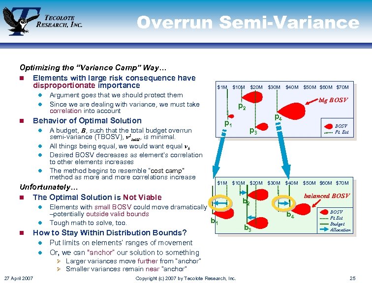
Overrun Semi-Variance Optimizing the “Variance Camp” Way… n Elements with large risk consequence have disproportionate importance l l n l l l A budget, B, such that the total budget overrun semi-variance (TBOSV), v 2 total, is minimal. All things being equal, we would want equal vk Desired BOSV decreases as element’s correlation to other elements increases The method begins to resemble “cost camp” method as more and more correlations increase Unfortunately… n The Optimal Solution is Not Viable l l $10 M Argument goes that we should protect them Since we are dealing with variance, we must take correlation into account $20 M $30 M $40 M p 4 p 1 $1 M $50 M $60 M $70 M big BOSV p 2 Behavior of Optimal Solution l n $1 M BOSV Pt. Est. p 3 $10 M Elements with small BOSV could move dramatically –potentially outside valid bounds b 1 Tough math to solve, too. How to Stay Within Distribution Bounds? $20 M $30 M $40 M balanced BOSV b 2 b 4 b 3 $50 M $60 M $70 M BOSV Pt. Est. Budget Allocation Put limits on elements’ ranges of movement l Or, we can “anchor” our solution to something l Ø Larger variances move further from “anchor” Ø Smaller variances remain near “anchor” 27 April 2007 Copyright (c) 2007 by Tecolote Research, Inc. 25

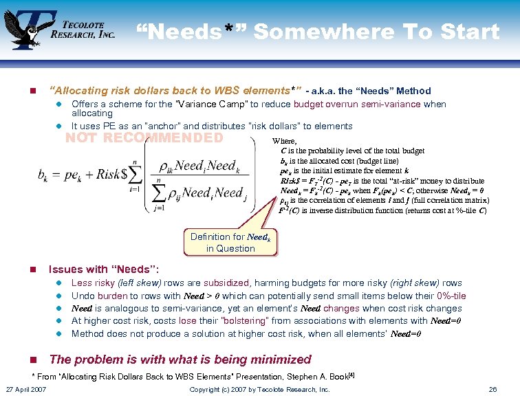
“Needs*” Somewhere To Start n “Allocating risk dollars back to WBS elements*” - a. k. a. the “Needs” Method l l Offers a scheme for the “Variance Camp” to reduce budget overrun semi-variance when allocating It uses PE as an “anchor” and distributes “risk dollars” to elements NOT RECOMMENDED Where, C is the probability level of the total budget bk is the allocated cost (budget line) pek is the initial estimate for element k Risk$ = FT-1(C) - pe. T is the total “at-risk” money to distribute Needk = Fk-1(C) - pek when Fk(pek) < C; otherwise Needk = 0 ρij is the correlation of elements i and j (full correlation matrix) F-1(C) is inverse distribution function (returns cost at %-tile C) Definition for Needk in Question n Issues with “Needs”: l l l n Less risky (left skew) rows are subsidized, harming budgets for more risky (right skew) rows Undo burden to rows with Need > 0 which can potentially send small items below their 0%-tile Need is analogous to semi-variance, yet an element’s Need changes when cost risk changes At higher cost risk, costs lose their “bolstering” from associations with elements with Need=0 Method does not produce a solution at higher cost risk, when all elements’ Need=0 The problem is with what is being minimized * From “Allocating Risk Dollars Back to WBS Elements” Presentation, Stephen A. Book[4] 27 April 2007 Copyright (c) 2007 by Tecolote Research, Inc. 26

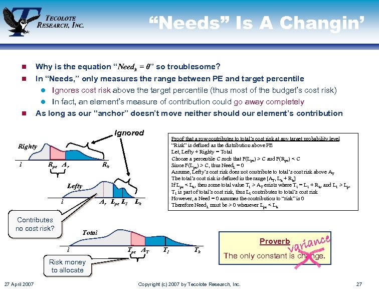
“Needs” Is A Changin’ n n n Why is the equation “Needk = 0” so troublesome? In “Needs, ” only measures the range between PE and target percentile l Ignores cost risk above the target percentile (thus most of the budget’s cost risk) l In fact, an element’s measure of contribution could go away completely As long as our “anchor” doesn’t move neither should our element’s contribution Ignored Proof that a row contributes to total’s cost risk at any target probability level “Risk” is defined as the distribution above PE Let, Lefty + Righty = Total Choose a percentile C such that F(Lpe) > C and F(Rpe) < C Since F(Lpe) > C, thus Need. L = 0 Assume, Lefty’s cost risk does not contribute to total’s cost risk above AT The total’s cost risk is defined in the range [AT, Lh + Rh] If Lpe < Lh, then some total value T 1 > AT exists where T 1 = L 1 + Rh, and L 1 > Lp, T 1 is part of total’s cost risk, thus L 1 contributes to total’s cost risk However, a Need = 0 assumes the contribution to “risk” is 0 Therefore Need. L must be > 0 whenever Lpe < Lh Righty l Rpe Ar Rh Lefty l Ar Lpe L 1 Contributes no cost risk? Total l Risk money to allocate 27 April 2007 Lh Tpe AT T 1 Th e ianc var Proverb The only constant is change. Copyright (c) 2007 by Tecolote Research, Inc. 27

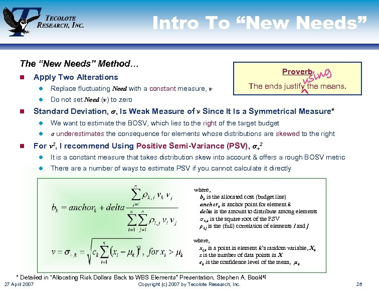
Intro To “New Needs” The “New Needs” Method… n l Replace fluctuating Need with a constant measure, v l n sing u Proverb Apply Two Alterations The ends justify the means. Do not set Need (v) to zero Standard Deviation, σ, Is Weak Measure of v Since It Is a Symmetrical Measure* l l n We want to estimate the BOSV, which lies to the right of the target budget σ underestimates the consequence for elements whose distributions are skewed to the right For v 2, I recommend Using Positive Semi-Variance (PSV), σ+2 l It is a constant measure that takes distribution skew into account & offers a rough BOSV metric l There a number of ways to estimate PSV if you cannot calculate it directly where, bk is the allocated cost (budget line) anchork is anchor point for element k delta is the amount to distribute among elements σ+, k is the square root of the PSV ρi, j is the (full) correlation of elements i and j where, xi, k is a point in element k’s random variable, Xk s is the number of data points in X ck is the confidence level of the mean, μk * Detailed in “Allocating Risk Dollars Back to WBS Elements” Presentation, Stephen A. Book[4] 27 April 2007 Copyright (c) 2007 by Tecolote Research, Inc. 28

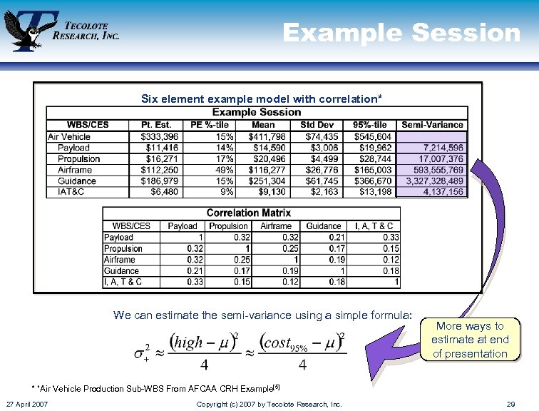
Example Session Six element example model with correlation* We can estimate the semi-variance using a simple formula: More ways to estimate at end of presentation * “Air Vehicle Production Sub-WBS From AFCAA CRH Example[5] 27 April 2007 Copyright (c) 2007 by Tecolote Research, Inc. 29

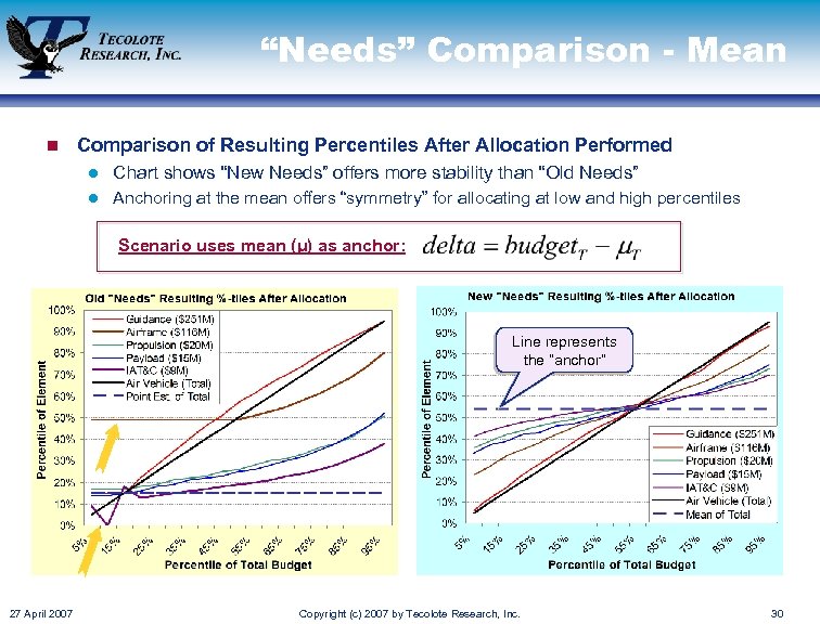
“Needs” Comparison - Mean n Comparison of Resulting Percentiles After Allocation Performed l Chart shows “New Needs” offers more stability than “Old Needs” l Anchoring at the mean offers “symmetry” for allocating at low and high percentiles Scenario uses mean (μ) as anchor: Line represents the “anchor” 27 April 2007 Copyright (c) 2007 by Tecolote Research, Inc. 30

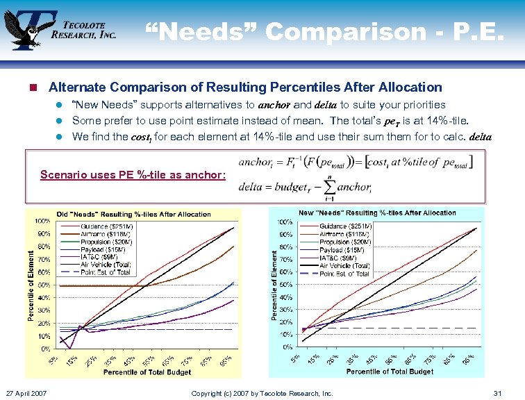
“Needs” Comparison - P. E. n Alternate Comparison of Resulting Percentiles After Allocation l “New Needs” supports alternatives to anchor and delta to suite your priorities l Some prefer to use point estimate instead of mean. The total’s pe. T is at 14%-tile. l We find the costi for each element at 14%-tile and use their sum them for to calc. delta Scenario uses PE %-tile as anchor: 27 April 2007 Copyright (c) 2007 by Tecolote Research, Inc. 31

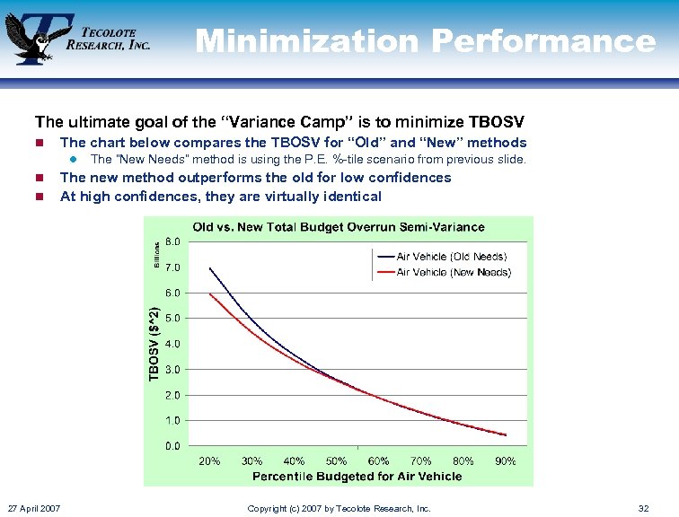
Minimization Performance The ultimate goal of the “Variance Camp” is to minimize TBOSV n The chart below compares the TBOSV for “Old” and “New” methods l n n The “New Needs” method is using the P. E. %-tile scenario from previous slide. The new method outperforms the old for low confidences At high confidences, they are virtually identical 27 April 2007 Copyright (c) 2007 by Tecolote Research, Inc. 32

Conclusion 27 April 2007 Copyright (c) 2007 by Tecolote Research, Inc. 33

In Conclusion n Cost Risk allocation is a tool that serves a specific purpose l Be sure that allocation serves your analysis goals l Only allocate when you have to encapsulate all money in WBS l Always allocate from where funds are managed l Allocate up or down the WBS n Two useful allocation methods were presented l Consider the two camps of thought when picking a method l How to minimize the total average budget overrun (TABO) l How to (nearly) reduce the total budget overrun semi-variance (TBOSV) Ø Introduction to a more reliable “New Needs” method to replace old one n Round to stress the (lack of) precision of your numbers n Be wary when discussing confidence levels after allocation l 27 April 2007 This is a huge topic on its own! Copyright (c) 2007 by Tecolote Research, Inc. 34

Questions? Contact Information John Sandberg ACEIT Master Programmer Tecolote Research, Inc. 5266 Hollister Ave. , Ste 301 Santa Barbara, CA 93109 Work: (805) 964 -6963 x 133 Fax: (805) 964 -7329 jsandberg@tecolote. com 27 April 2007 Copyright (c) 2007 by Tecolote Research, Inc. 35

References: [1] Information on the meanings of accuracy and precision: http: //en. wikipedia. org/wiki/Accuracy_and_precision http: //en. wikipedia. org/wiki/Significance_arithmetic#Uncertainty_and_error [2] Examples of rounding at 2 nd decimal of deviation: http: //physics. nist. gov/cuu/Constants/ Description of Semi-Variance [3] “Selected Semi-Variance Estimators of Underreporting Non. Farm Sole Proprietor Income, ” Chih. Chin Ho, Internal Revenue Service, IRC 1996_028 http: //www. amstat. org/sections/srms/proceedings/papers/1996_028. pdf Detailed description of the “Needs” method and model [4] “Allocating Risk Dollars Back to WBS Elements” Stephen A. Book, Chief Technical Officer, MCR, LLC SSCAG/EACE/SCAF Meeting 19 -21 September 2006, also presented at SCEA Conference June 2006, Do. DCAS Symposium February 2007 Additional information on uncertainty analysis and time-phased cost risk allocation [5] “AFCAA Cost Risk Handbook” Alfred Smith et. al. , CR-1254 -3, 9 April [6] “’Need’ Needs Kneading” John Sandberg, Tecolote Research, Inc. , presented at SSCAG Meeting 17 Jan 2007 27 April 2007 Copyright (c) 2007 by Tecolote Research, Inc. 36

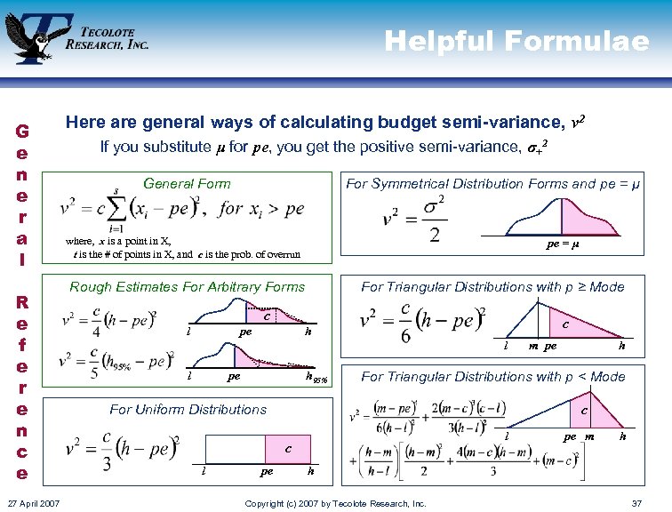
Helpful Formulae G e n e r a l R e f e r e n c e 27 April 2007 Here are general ways of calculating budget semi-variance, v 2 If you substitute μ for pe, you get the positive semi-variance, σ+2 General Form For Symmetrical Distribution Forms and pe = μ where, x is a point in X, t is the # of points in X, and c is the prob. of overrun pe = μ Rough Estimates For Arbitrary Forms For Triangular Distributions with p ≥ Mode c l pe c h l l pe h 95% c l c pe h For Triangular Distributions with p < Mode For Uniform Distributions l m pe pe m h h Copyright (c) 2007 by Tecolote Research, Inc. 37

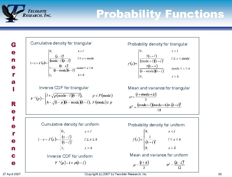
Probability Functions G e n e r a l R e f e r e n c e 27 April 2007 Cumulative density for triangular Inverse CDF for triangular Cumulative density for uniform Inverse CDF for uniform Probability density for triangular Mean and variance for triangular Probability density for uniform Mean and variance for uniform Copyright (c) 2007 by Tecolote Research, Inc. 38

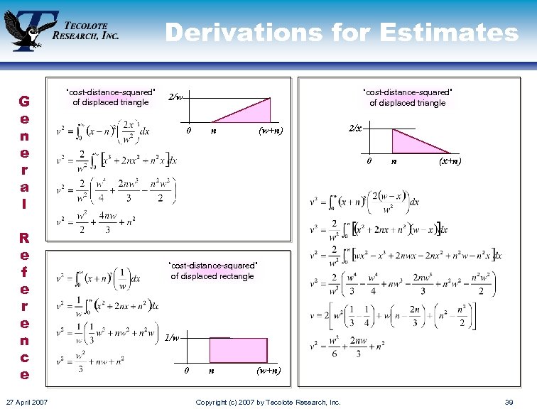
Derivations for Estimates G e n e r a l R e f e r e n c e 27 April 2007 “cost-distance-squared” of displaced triangle 2/w 0 n (w+n) 2/x 0 n (x+n) “cost-distance-squared” of displaced rectangle 1/w 0 n (w+n) Copyright (c) 2007 by Tecolote Research, Inc. 39

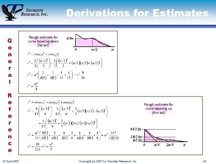
Derivations for Estimates G e n e r a l R e f e r e n c e 27 April 2007 Rough estimate for curve tapering down (fat tail) 4/3 w 0 w/2 w Rough estimate for curve tapering up (thin tail) 54/13 x 18/13 x 6/13 x 0 Copyright (c) 2007 by Tecolote Research, Inc. x/3 2 x/3 x 40