Cosmology the Big Bang AY 16 Lecture

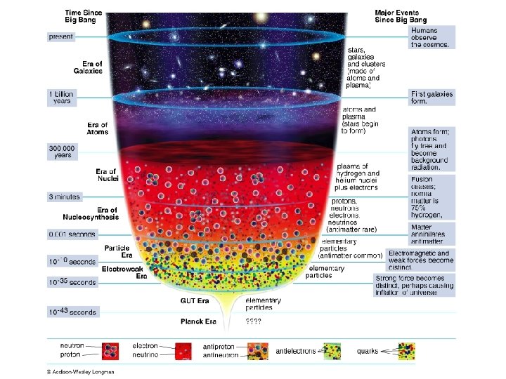
Cosmology & the Big Bang AY 16 Lecture 20, April 15, 2008 Mathematical Cosmology, con’t Determination of Cosmological Parameters Inflation & the Big Bang

Einstein’s Equations: 2 2 2 (d. R/dt) /R + kc /R = 8 p. Ge/3 c +Lc /3 2 energy density 2 2 CC 2 2(d R/dt )/R + (d. R/dt) /R + kc /R = -8 p. GP/c +Lc 3 pressure term 2

And Friedmann’s Equations: 2 2 2 (d. R/dt) = 2 GM/R + Lc R /3 – kc 2 2 Ro [(8 p. G/3)ro – Ho] if L = 0 (no Cosmological Constant) 2 2 kc = or 2 (d. R/dt) /R - 8 p. Gro /3 =Lc /3 – kc which is known as Friedmann’s Equation 2 /R 2

Note that if we assume Λ = 0, we have (d 2 R/dt 2)/R = - 4πG (ρ + 3 P) 3 and in a matter dominated Universe, ρ >> P So we can define a critical density by combining the cosmological equations: 3 ρC = 8πG . 2 3 H 02 R = R 2 8πG

And we define the ratio of the density to the critical density as the parameter Ω ≡ ρ/ρC For a matter dominated, Λ=0 cosmology, Ω > 1 = closed Ω = 1 = flat, just bound Ω < 1 = open There are many possible forms of R(t), especially when Λ and P are reintroduced. Its our job to find the right one!

Λ=0

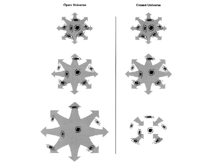
Some of possible forms are: Big Bang Models: Einstein-de. Sitter k=0 flat, open & infinite expands Friedmann-Lemaitre k=-1 hyperbolic “ “ “ k=+1 spherical, closed finite, collapses Leimaitre Λ ≠ 0 k=+1 spherical, closed finite, expands

Non-Big Bang Models Eddington-Lemaitre Λ≠ 0 k=+1 spherical, closed, finite, static then expands Steady State k=0 flat, open, infinite, stationary de. Sitter k=0 empty, no singularity, open, infinite H 02 (Ω 0 – 1) + 1/3 Λ 0 k= c 2 ≡ Radius of Curvature of the Universe

R(t) A Child’s Garden E-L F-L, 0 Ed. S of Cosmological Models SS, d. S L F-L, C t

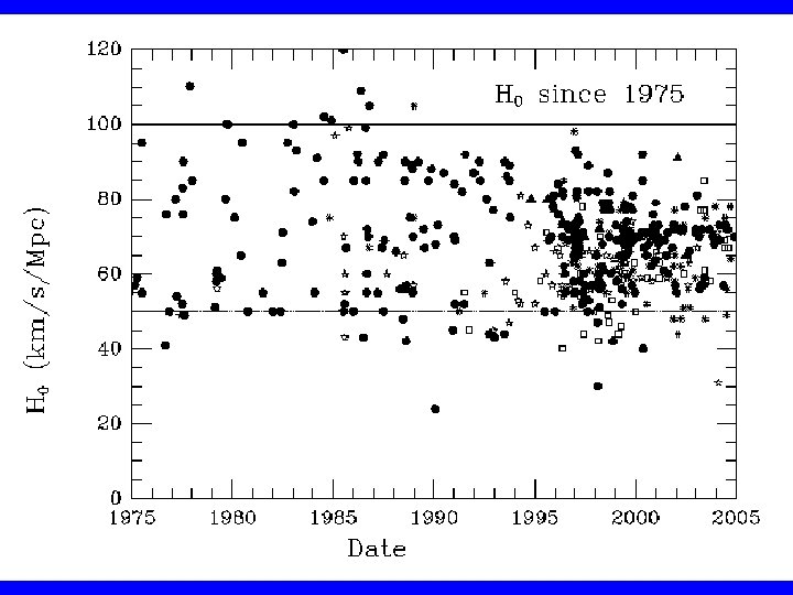
Cosmology is now the search for three numbers: • The Expansion Rate = Hubble’s Constant = H 0 • The Mean Matter Density = Ωmatter • The Cosmological Constant = ΩΛ Taken together, these three numbers describe the geometry of space-time and its evolution. They also give you the Age of the Universe.

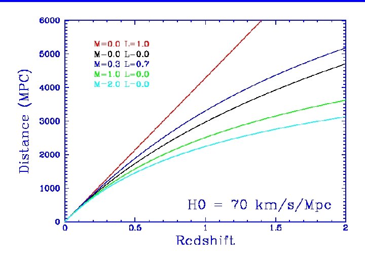
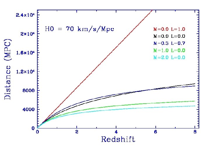
Lookback Time For a Friedmann-Lemaitre Big-Bang Model, the lookback time as a function of redshift is τL = H 0 -1 z ( 1+z ) for q 0=0; Λ=0 = 2/3 H 0 -1 [1 – (1 + z)-3/2] for q 0=1/2, Λ=0

The Hubble Constant: • H 0 = *current* expansion rate • • = (velocity) / (distance) = (km/s) / (Megaparsecs) • named after Edwin Hubble who discovered the relation in 1929.

The story of the Hubble Constant (never called that by Hubble!) is the “Cosmological Distance Ladder” or the “Extragalactic Distance Scale” Basically, we need distances & velocities to galaxies and other things. Velocities are easy --- pick a galaxy, any galaxy, get spectrum with moderate resolution, R ~ 1000 (i. e λ/R ~ 5Å) N. B. R = Linear Reciprocal Dispersion, get line centroids to ~ 1/10 R ~ 0. 5Å/5000Å ~ 1 part in 104 ~ 30 km/s

Spectral features in galaxies

Velocity Measurement Radial Velocities (stars, galaxies) now usually measured by cross-correlation techniques pioneered by Simkin (1973), Schechter (1976) & Tonry & Davis (1979). Accuracy depends on Signal-to-Noise and resolution. Typically, for S/N > ~ 20, errors are ~ 10% of Δλ, where (remember) R = λ/Δλ

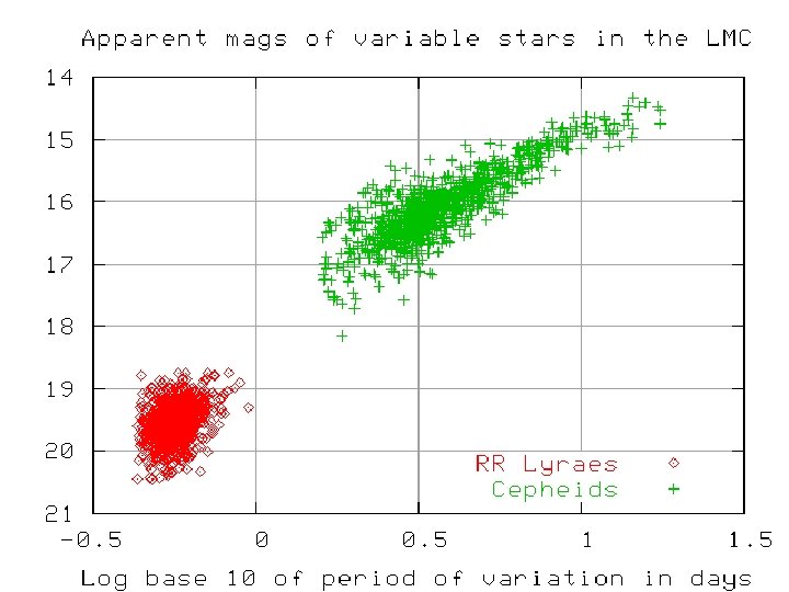
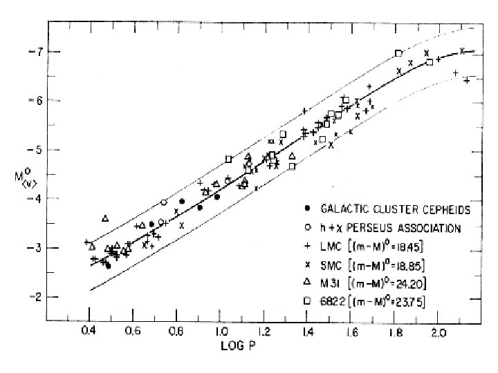
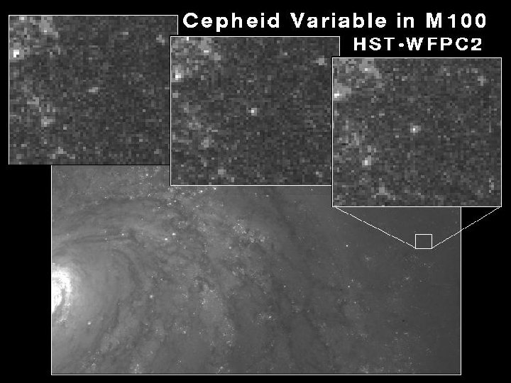
Distances are Hard! Hubble’s original estimates of galaxy distances were based on brightest stars which were based on Cepheid Variables Distances to the LMC, SMC, NGC 6822 & eventually M 31 from Cepheids. Find the brightest stars and assume they’re the same (independent of galaxy type, etc. )

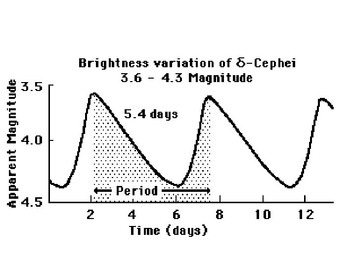
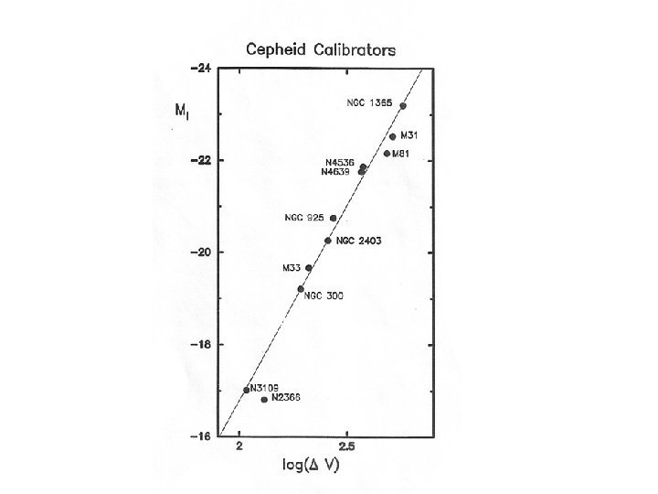
Cepheids Pretty Good Distance Indicators --- Standard Candles from the Period-Luminosity (PL) relation: L ≈ P 3/2 PLC relation MV = -2. 61 - 3. 76 log P +2. 60 (B-V) but ya gotta find them! H 0 circa 1929 ~ 600 km/s/Mpc Wrong! 1. Hubble’s galactic calibrators not classical Cepheids. 2. At large distances, brightest stars confused with star clusters. 3. Hubble’s magnitude scale was off.

• P-L Relation, LMC

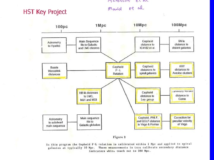
de. Vaucouleurs ‘ 76 Cosmological Distance Ladder

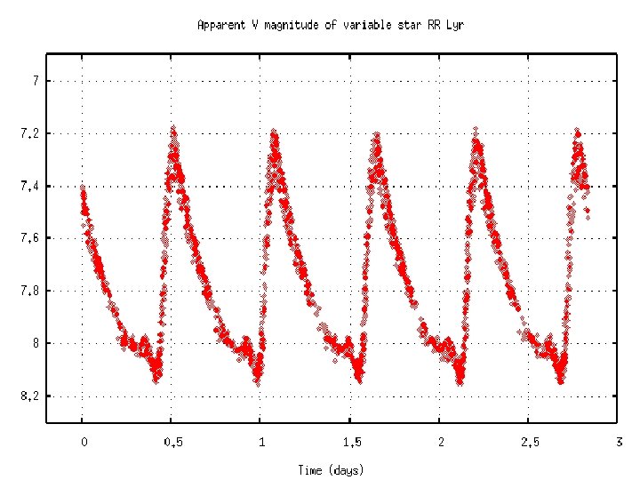
Cosmological Distance Ladder Find things that work as distance indicators (standard candles, standard yardsticks) to greater and greater distances. Locally: Primary Indicators Cepheids MB ~ -2 to -6 RR Lyrae Stars MB ~ 0 Novae MB ~ -6 to -9

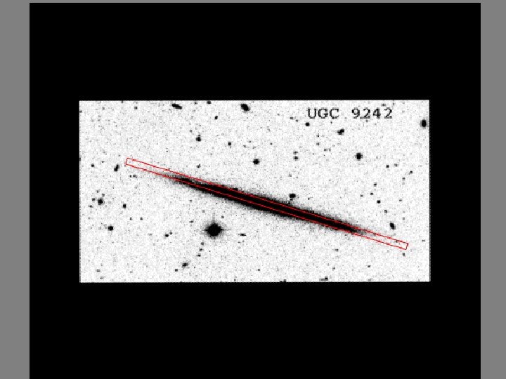
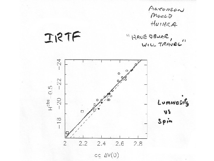
Calibrate Cepheids via parallax, moving cluster = convergent point method, expansion parallax Baade-Wesselink, main sequence (HR diagram) fitting. Secondary Distance Indicators Brightest Stars (XX? ? ) Tully-Fisher (+ IRTF) Planetary Nebulae LF Globular Cluster LF

Supernovae of type Ia Supernovae of type II (EPM) Fundamental Plane (Dn-σ) Faber-Jackson Surface Brightness Fluctuations Red Giant Branch Tip Luminosity Classes (XXX) HII Region Diameters (XXX) HII Region Luminosities (? ? ? )

Lemaitre 1927 Hubble 1929 Oort 1932 Baade 1952

• Tully-Fisher

Surface Brightness Fluctuations Tonry & Schneider

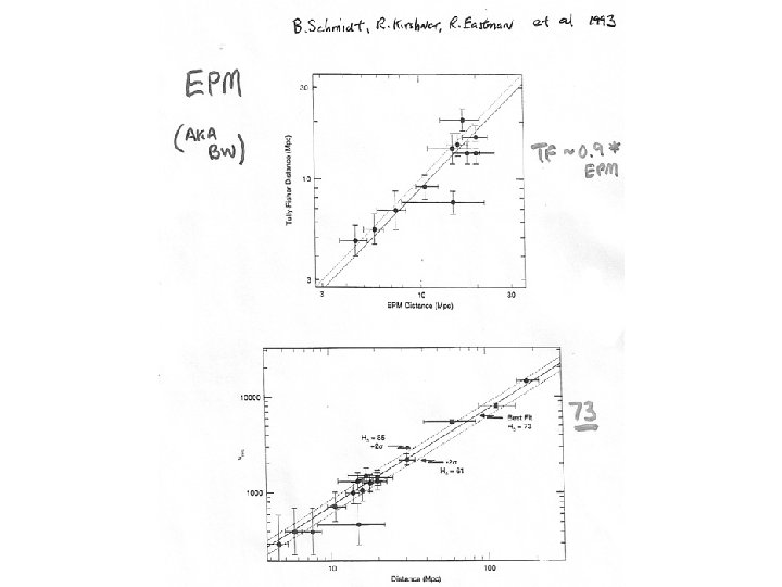
Baade-Wesselink --- EPM = Expanding Photospheres Method Basically observe and expanding/contracting object at two (multiple) times. Get redshift and get SED. Then L 1 = 4πR 12σT 14 & L 2 = 4πR 22σT 24 and R 2 = R 1 + v δt (or better ∫ vdt)

Fukugita, Hogan & Peebles 1993

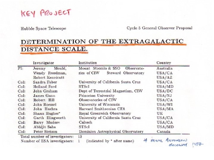
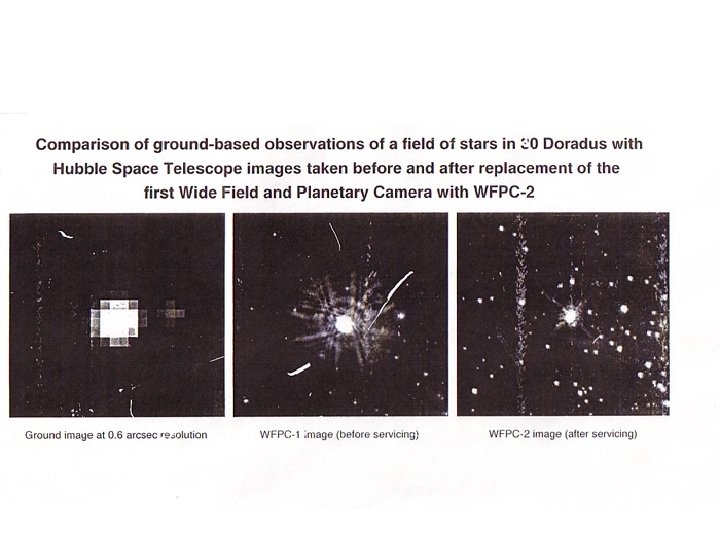
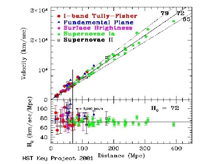
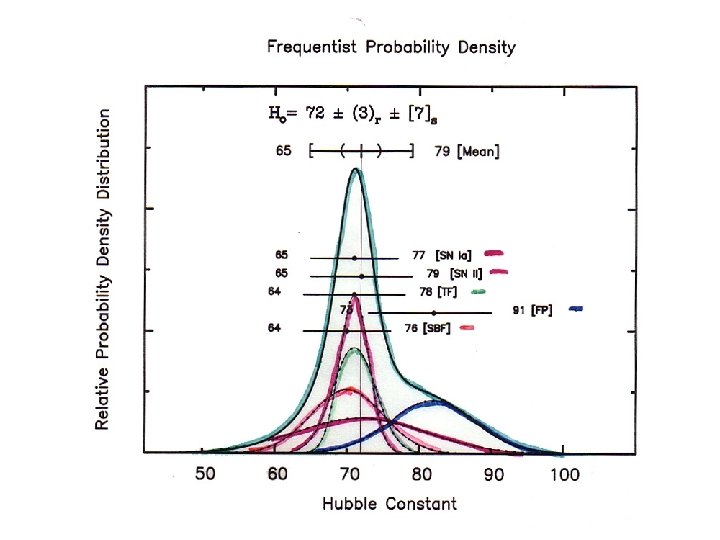
HST H 0 Key Project Team •

WFPC 2 footprint

Cepheid Light Curves N 1326 a

Matching P-L Relations IC 4182 (HST) MW (Ground)

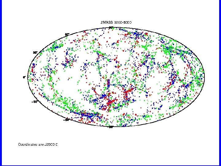
(matter): 0. Baryons from Nucleosynthesis 1. Sum up Starlight (count stars and/ or count galaxies) 2. Count and Weigh Galaxies 3. Use Global techniques: Large Scale Structure Large Scale Flows

Big Bang Nucleosynthesis

For H 0=70 km/s/Mpc (baryons) ~ 0. 04

Ωmatter: Measure luminosity density = (sum of all galaxies x their luminosity) per unit volume (l/v) = L Measure mean mass-to-light ratio for galaxies (M/L) Multiply: Mass density = (M /L) x (L) How do we measure the Luminosity density?

Redshift Surveys + Φ(M) Measure the Galaxy Luminosity Function For a typical flux (magnitude = m. L) limited survey, we can see a galaxy of absolute magnitude M to a distance r = 10 ( m. L -M - 25)/5 Mpc V(M) = 4/3 π r 3 (Survey Solid Angle) then Φ(M) = d. N(M)/d. M = N(M, M±d. M/2)/V(M)

Φ(M) or Φ(L) is the number density of galaxies of a given magnitude or luminosity in a sample. Early forms: Zwicky Hubble N Holmberg M

Abell Form (circa 1960) = two power laws Now use the Schechter LF Form: α exp(-L/L*) d(L/L*) Φ(L) d. L = φ* (L/L*) or Φ(M)d. M = 0. 4 φ* log[dex 0. 4(M*-M)]α+1 exp[-dex 0. 4(M*-M)] d. M where φ* = normalization (# / Mpc 3) α = faint end slope M*, L* = characteristic mag or luminosity

Schechter Form The Schechter form for the LF is derived from Press-Schechter formalism for self-similar galaxy formation (more later). Is integrable(!) solution: L = φ* L* Γ(α+2) a Gamma function

Galaxy Luminosity Function:

Luminosity Density The Luminosity Density is then just the integral of the luminosity function: ∞ L= or L= ∫ 0 ∫ L Φ(L) d. L ∞ 0 L(M) Φ(M) d. M (either way works)

Luminosity Density Typical numbers: B band R band K band log L = 26. 65 log L = 26. 90 log L = 27. 20 ergs s-1 Hz-1 Mpc-3 for H 0=70, 8 L / Mpc 3 in Solar Units LB = 1. 2 x 10 In units of

Galaxy Masses and M/Ls Galaxies are weighed via a large number of techniques: (a) Disk Dispersion (more later) (b) Rotation Curves (c) Velocity Dispersions (d) Binary Galaxies (e) Galaxy Groups

(f) Galaxy Clusters Virial Theorem /Projected Mass Hydrostatic Equilibrium Gravitational Lensing (g) Large Scale Flows (e) Cosmic Virial Theorem Galaxy Field Velocity Dispersion In all cases, L = Σ LGal in the system.

(b) Rotation Curves ½ m 1 v(r)2 (sin i)2 GM(r)m 1 r = v(r)2 r M(r) = G 2 r 2 (sin i)2 With m 1 = test particle mass, i = inclination, r = radius, v(r) = rotation speed at r

(d) Binary Galaxies Must Model Projection Effects! M ~ 1 cos 3 i cos 2φ i = inclination angle φ = orbital velocity angle

Abell 2142 Hot Gas in X-rays

Strong Gravitational Lensing

Galaxy Flows: Observed galaxy “velocity” is composed of several parts VO = VHubble + Vpeculiar + Vgrav + LSR and VP/VH = (1/3) (dr/r) 0. 66

• Blue 1000 < V < 2000 km/s VIRGO • The Local Supercluster

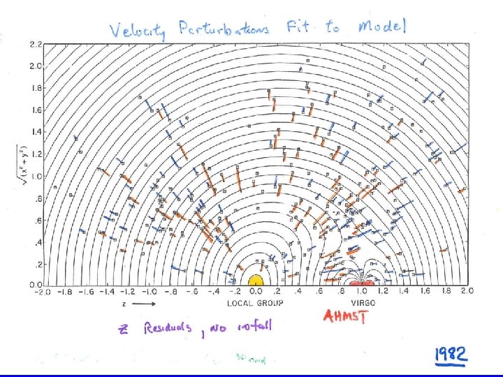
The Local Supercluster We have an infall measure for the LSC and from redshift surveys we have a pretty good measure of δρ/ρ: VP ~ 250 km/s VH = 1100 + 250 km/s = 1350 δρ/ρ ~ 2. 5 Ω ~ 0. 25

In terms of M/LB Ratios M/L populations M/L rotation/dispersion M/L galaxy satellites M/L binaries M/L galaxy groups M/L Clusters M/L CVT M/L Flows ~ 1 -5 ~ 10 ~ 25 ~ 50 ~ 100 ~ 400 ~ 3 -500 ~ 500

What’s This Saying? (1) M/L maxes out ~ 450, ΩG = ΩM = 0. 25 ± 0. 05 (2) M/L grows with scale? ! Gravitating matter seems to be distributed on a scale somewhat larger than galaxies. and there’s more of it than Baryons Non-Baryonic Dark Matter exists

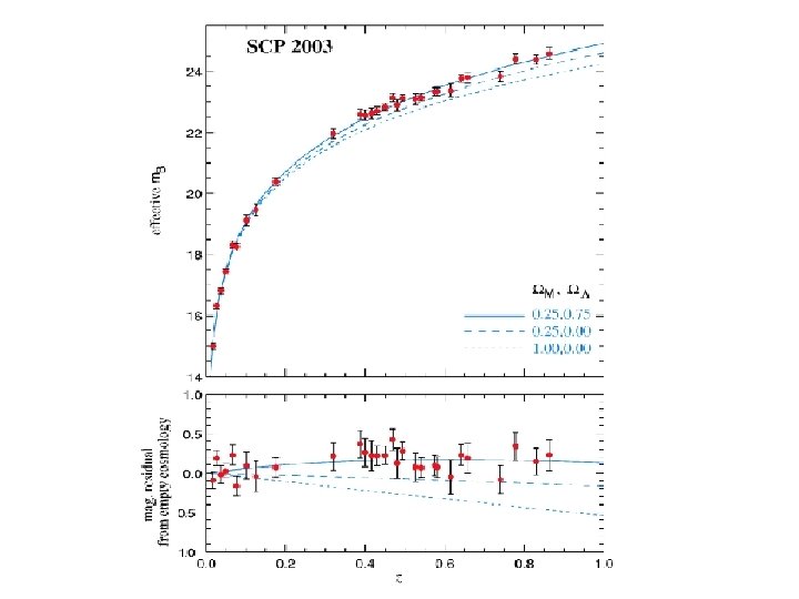
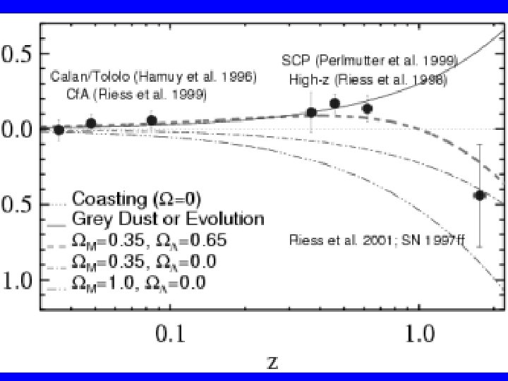
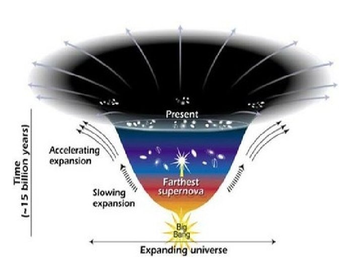
Cosmological Constant: Cosmological Constant = Lambda is measured by observing the geometry of the Universe at large redshift (distance) Supernovae as standard candles CMB Fluctuations vs Models

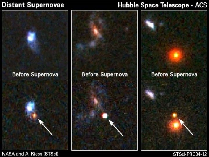
Essence Project, 2004

Levels of Certainty in Science You bet: A Dime = $0. 1 Your Dog = $100 Your House = $100, 000 Your Firstborn = $100, 000 …. each x 1000 (except in New York and Boston where everything is x 10!!!)

WMAP Microwave Sky

Best Fit b=0. 04 CDM=0. 27 L=0. 71 T=1. 02 +/- 0. 02

Large scale geometry: CMB Fluctuations as measured by WMAP indicate that ΩT is very nearly unity (1. 02 +/- 0. 02) the Universe is FLAT ΩΛ = ΩT - ΩM

Contents: = (density of the Universe)/ (closure density) = 1. 02 +/- 0. 02 + (total) = (baryons) + (neutrinos) + (Cold dark matter) (Dark Energy)

Contents: Omega (stars) =0. 005 +/- 0. 002 Omega(baryons) = 0. 044 +/- 0. 004 Omega(neutrinos) < 0. 008 Omega(CDM) = 0. 23 +/- 0. 04 Omega(Dark Energy) = 0. 73 +/- 0. 04 Omega(Total) = 1

Contents of the Universe

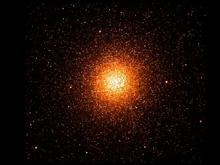
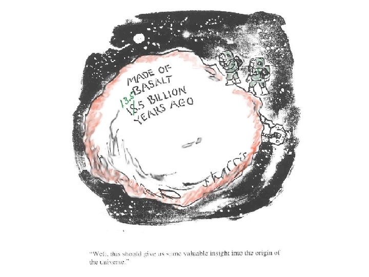
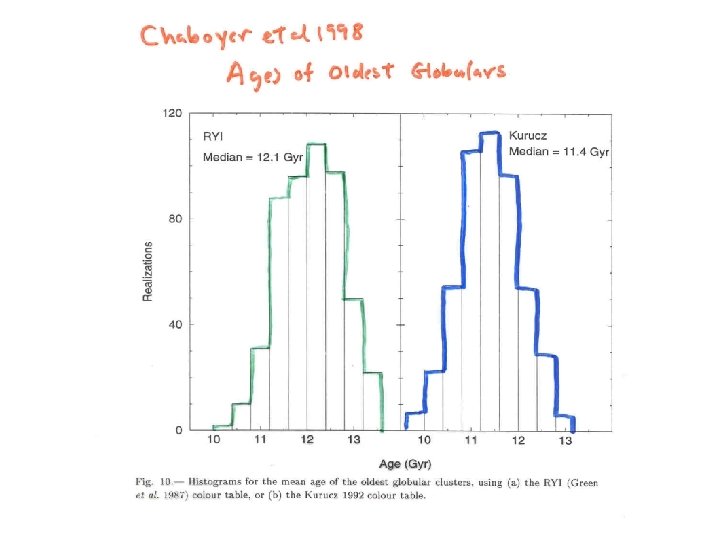
Age of the Universe: Ages of the Oldest things: stars, galaxies, star clusters Cosmological expansion age : ~ (1/H 0) x geometric factors

Cosmological Age Calculation In FRW Cosmologies, the age of the Universe is calculated from τ0 = -H 0 -1 ∫ 0 ∞ dz (1+z)[(1+z)2(ΩMz+1) – ΩΛz(z+2)]1/2 Where the terms are fairly self explanatory. We need to know H 0, ΩM and ΩΛ

The empty model has t 0 = H 0 -1 The SCDM Flat model has t 0 = (2/3) H 0 -1 For the general case (with a CC), the full form is: and a good approximation is t 0 = -1 -1 1/2 (2/3) H 0 sinn [(|1 - a|/ a) ] / |[1 - a]| 1/2

Where a = matter -0. 3* total + 0. 3 and sinn-1 = sinh-1 = sin -1 a </= 1 if a > 1 if (from Carroll, Press and Turner, 1992) Also, for a flat model with L, t 0 = -1 (2/3)H 0 L -1/2 ln[(1+ L 1/2 )/(1 - L) 1/2 ]

The Age of Flat Universes H 0/ΩΛ 0. 0 0. 6 0. 7 0. 8 55 65 70 75 11. 9 10. 0 9. 4 8. 7 15. 1 12. 7 11. 9 11. 1 17. 1 14. 5 13. 6 12. 6 18. 5 16. 2 15. 1 14. 0 Where Ωtotal = 1. 00000, and the ΩΛ = 0 models are the Standard CDM models in Gyr

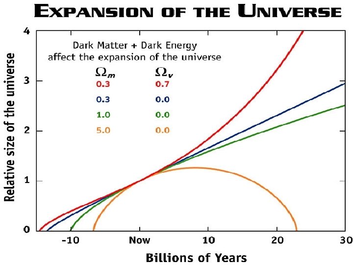
Alternatives ΩM = 0. 3, ΩΛ = 0 gives τ0 = 0. 79 H 0 -1 = 11. 8 Gyr for H=65 (no Lambda) ΩM = 0. 25, ΩΛ = 0. 6 gives τ0 = 0. 97 H 0 -1 = 14. 6 Gyr for H=65 (minimal Lambda)

JPH’s Favorite Guess Today: H 0 = 70 +/- 5 km/s/Mpc The Universe is going to expand forever Its current age is around 14 Billion Years, and There is a good chance its FLAT with a Cosmological constant = (Lambda) ~ 0. 7