b91403eb22c0cebc19973020f116166d.ppt
- Количество слайдов: 38

Copyright © 2009 Pearson Education, Inc. Publishing as Prentice Hall. 1 of 22 Macroeconomics: Principles, Applications, and Tools O’Sullivan, Sheffrin, Perez 6/e.

Copyright © 2009 Pearson Education, Inc. Publishing as Prentice Hall. 2 of 22 Macroeconomics: Principles, Applications, and Tools O’Sullivan, Sheffrin, Perez 6/e.

6/e. O’Sullivan, Sheffrin, Perez Macroeconomics: Principles, Applications, and Tools The Income-Expenditure Model By 2003, the Japanese economy appeared to have recovered from a recession that began in the early 1990 s. PREPARED BY FERNANDO QUIJANO, YVONN QUIJANO, AND XIAO XUAN XU Copyright © 2009 Pearson Education, Inc. Publishing as Prentice Hall. 3 of 22
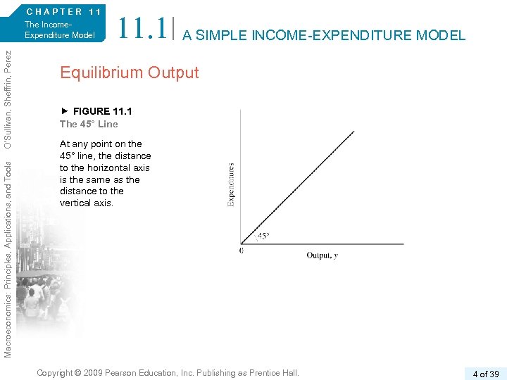
Macroeconomics: Principles, Applications, and Tools O’Sullivan, Sheffrin, Perez 6/e. CHAPTER 11 The Income. Expenditure Model 11. 1 A SIMPLE INCOME-EXPENDITURE MODEL Equilibrium Output FIGURE 11. 1 The 45° Line At any point on the 45° line, the distance to the horizontal axis is the same as the distance to the vertical axis. Copyright © 2009 Pearson Education, Inc. Publishing as Prentice Hall. 4 of 39
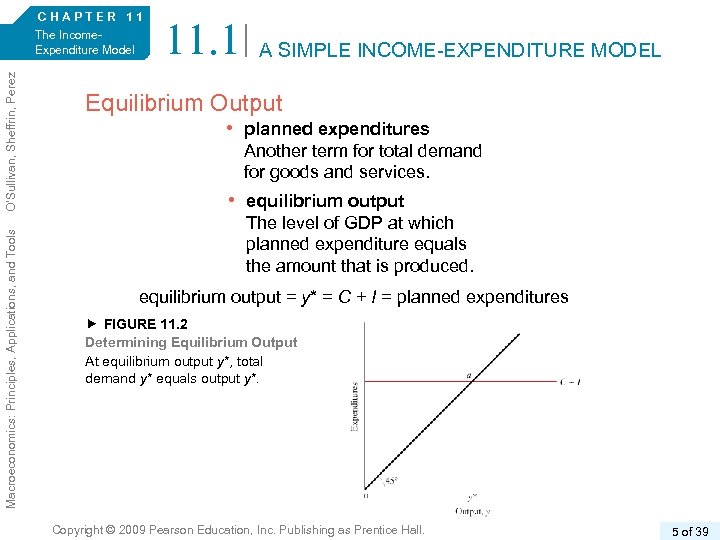
Macroeconomics: Principles, Applications, and Tools O’Sullivan, Sheffrin, Perez 6/e. CHAPTER 11 The Income. Expenditure Model 11. 1 A SIMPLE INCOME-EXPENDITURE MODEL Equilibrium Output • planned expenditures Another term for total demand for goods and services. • equilibrium output The level of GDP at which planned expenditure equals the amount that is produced. equilibrium output = y* = C + I = planned expenditures FIGURE 11. 2 Determining Equilibrium Output At equilibrium output y*, total demand y* equals output y*. Copyright © 2009 Pearson Education, Inc. Publishing as Prentice Hall. 5 of 39
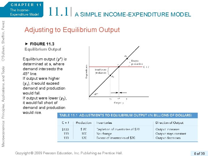
Macroeconomics: Principles, Applications, and Tools O’Sullivan, Sheffrin, Perez 6/e. CHAPTER 11 The Income. Expenditure Model 11. 1 A SIMPLE INCOME-EXPENDITURE MODEL Adjusting to Equilibrium Output FIGURE 11. 3 Equilibrium Output Equilibrium output (y*) is determined at a, where demand intersects the 45° line. If output were higher (y 1), it would exceed demand production would fall. If output were lower (y 2), it would fall short of demand production would rise. Copyright © 2009 Pearson Education, Inc. Publishing as Prentice Hall. 6 of 39
Macroeconomics: Principles, Applications, and Tools O’Sullivan, Sheffrin, Perez 6/e. CHAPTER 11 The Income. Expenditure Model 11. 2 THE CONSUMPTION FUNCTION Consumer Spending and Income • consumption function The relationship between consumption spending and the level of income. C = Ca + by • autonomous consumption The part of consumption that does not depend on income. • marginal propensity to consume (MPC) The fraction of additional income that is spent. Copyright © 2009 Pearson Education, Inc. Publishing as Prentice Hall. 7 of 39
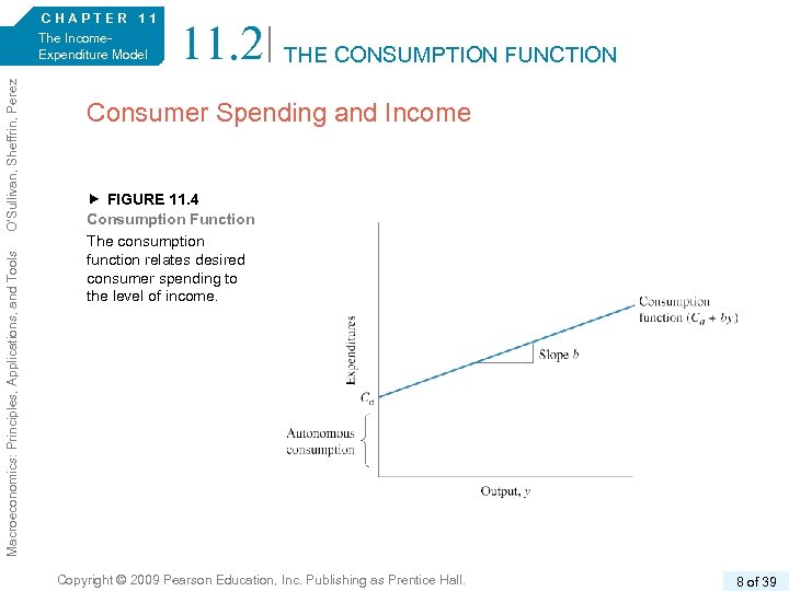
Macroeconomics: Principles, Applications, and Tools O’Sullivan, Sheffrin, Perez 6/e. CHAPTER 11 The Income. Expenditure Model 11. 2 THE CONSUMPTION FUNCTION Consumer Spending and Income FIGURE 11. 4 Consumption Function The consumption function relates desired consumer spending to the level of income. Copyright © 2009 Pearson Education, Inc. Publishing as Prentice Hall. 8 of 39
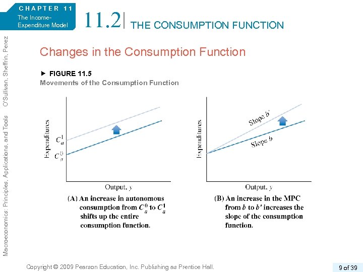
The Income. Expenditure Model 11. 2 THE CONSUMPTION FUNCTION Changes in the Consumption Function FIGURE 11. 5 Movements of the Consumption Function Macroeconomics: Principles, Applications, and Tools O’Sullivan, Sheffrin, Perez 6/e. CHAPTER 11 Copyright © 2009 Pearson Education, Inc. Publishing as Prentice Hall. 9 of 39
Macroeconomics: Principles, Applications, and Tools O’Sullivan, Sheffrin, Perez 6/e. CHAPTER 11 The Income. Expenditure Model 11. 2 THE CONSUMPTION FUNCTION Changes in the Consumption Function Two factors that can cause autonomous consumption to change: • Increases in consumer wealth will cause an increase in autonomous consumption. • Increases in consumer confidence will increase autonomous consumption. Copyright © 2009 Pearson Education, Inc. Publishing as Prentice Hall. 10 of 39

6/e. O’Sullivan, Sheffrin, Perez Macroeconomics: Principles, Applications, and Tools CHAPTER 11 The Income. Expenditure Model APPLICATION 1 FALLING HOME PRICES, THE WEALTH EFFECT, AND DECREASED CONSUMER SPENDING APPLYING THE CONCEPTS #1: How do changes in the value of homes affect consumer spending? The value of homes in excess of what people borrow with a mortgage is known as their home equity. Home equity is the single largest component of net wealth for most families in the United States. Changes in the value of home equity—like other forms of wealth—affect consumer spending. The period from 1997 to mid-2006 was paradise for consumers. Housing prices rose nationally by approximately 90 percent and consumer wealth grew by $6. 5 trillion dollars over that period. The party ended in the summer of 2006 as housing prices began to fall. In its review of the literature, the Congressional Budget Office found most studies estimated a decrease of consumer wealth of $1 would lower consumption spending by somewhere between $. 02 and $. 07, or ultimately from $21 to $72 billion of spending. This decrease would subtract 0. 1 to 0. 5 percentage points from economic growth during 2007. Copyright © 2009 Pearson Education, Inc. Publishing as Prentice Hall. 11 of 39
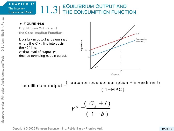
Macroeconomics: Principles, Applications, and Tools O’Sullivan, Sheffrin, Perez 6/e. CHAPTER 11 The Income. Expenditure Model 11. 3 EQUILIBRIUM OUTPUT AND THE CONSUMPTION FUNCTION FIGURE 11. 6 Equilibrium Output and the Consumption Function Equilibrium output is determined where the C + I line intersects the 45° line. At that level of output, y*, desired spending equals output. Copyright © 2009 Pearson Education, Inc. Publishing as Prentice Hall. 12 of 39
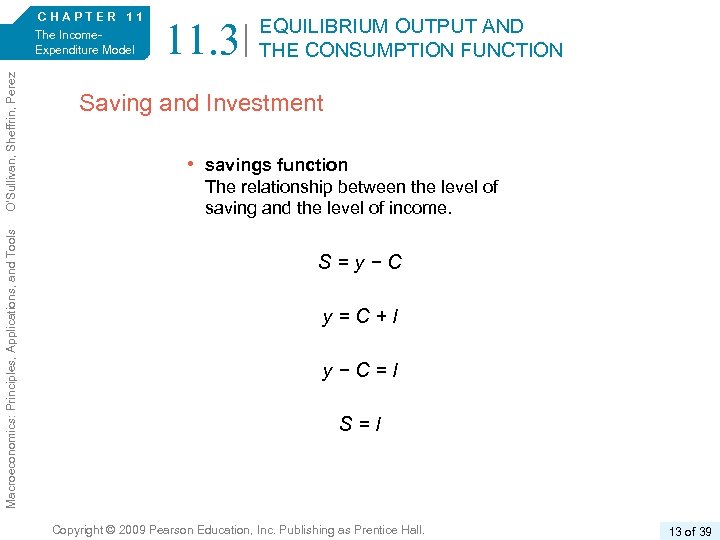
Macroeconomics: Principles, Applications, and Tools O’Sullivan, Sheffrin, Perez 6/e. CHAPTER 11 The Income. Expenditure Model 11. 3 EQUILIBRIUM OUTPUT AND THE CONSUMPTION FUNCTION Saving and Investment • savings function The relationship between the level of saving and the level of income. S=y−C y=C+I y−C=I S=I Copyright © 2009 Pearson Education, Inc. Publishing as Prentice Hall. 13 of 39
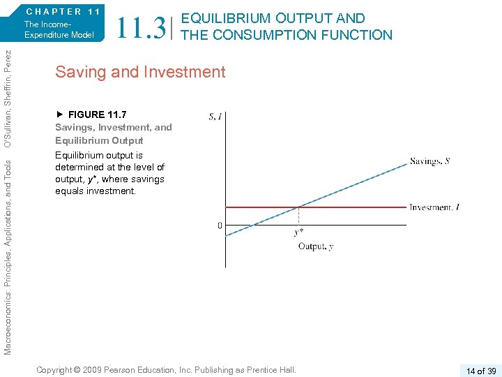
Macroeconomics: Principles, Applications, and Tools O’Sullivan, Sheffrin, Perez 6/e. CHAPTER 11 The Income. Expenditure Model 11. 3 EQUILIBRIUM OUTPUT AND THE CONSUMPTION FUNCTION Saving and Investment FIGURE 11. 7 Savings, Investment, and Equilibrium Output Equilibrium output is determined at the level of output, y*, where savings equals investment. Copyright © 2009 Pearson Education, Inc. Publishing as Prentice Hall. 14 of 39
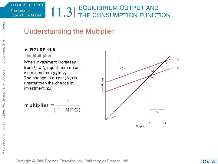
Macroeconomics: Principles, Applications, and Tools O’Sullivan, Sheffrin, Perez 6/e. CHAPTER 11 The Income. Expenditure Model 11. 3 EQUILIBRIUM OUTPUT AND THE CONSUMPTION FUNCTION Understanding the Multiplier FIGURE 11. 8 The Multiplier When investment increases from I 0 to I 1, equilibrium output increases from y 0 to y 1. The change in output (Δy) is greater than the change in investment (ΔI). Copyright © 2009 Pearson Education, Inc. Publishing as Prentice Hall. 15 of 39
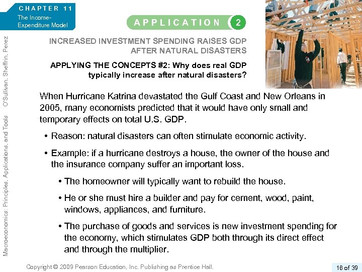
Macroeconomics: Principles, Applications, and Tools O’Sullivan, Sheffrin, Perez 6/e. CHAPTER 11 The Income. Expenditure Model APPLICATION 2 INCREASED INVESTMENT SPENDING RAISES GDP AFTER NATURAL DISASTERS APPLYING THE CONCEPTS #2: Why does real GDP typically increase after natural disasters? When Hurricane Katrina devastated the Gulf Coast and New Orleans in 2005, many economists predicted that it would have only small and temporary effects on total U. S. GDP. • Reason: natural disasters can often stimulate economic activity. • Example: if a hurricane destroys a house, the owner of the house and the insurance company suffer an important loss. • The homeowner will typically want to rebuild the house. • He or she must hire a builder and pay for cement, wood, paint, windows, appliances, and furniture. • The purchase of goods and services is new investment spending for the economy, which stimulates GDP both through its direct effect and through the multiplier. Copyright © 2009 Pearson Education, Inc. Publishing as Prentice Hall. 16 of 39
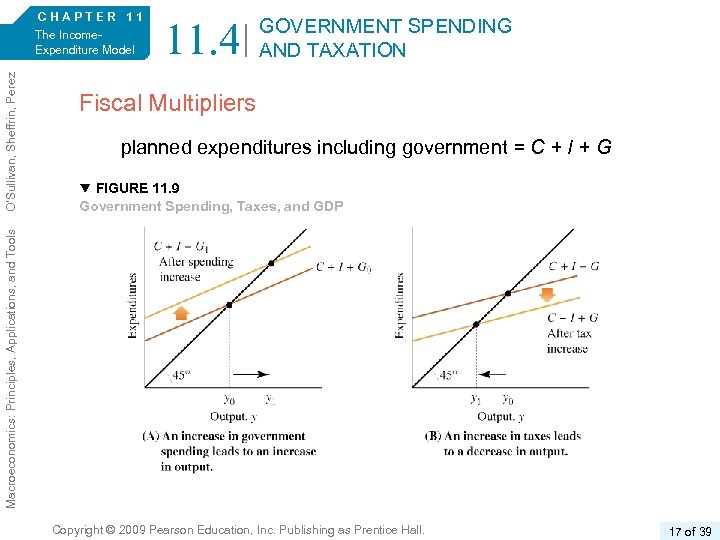
The Income. Expenditure Model 11. 4 GOVERNMENT SPENDING AND TAXATION Fiscal Multipliers planned expenditures including government = C + I + G FIGURE 11. 9 Government Spending, Taxes, and GDP Macroeconomics: Principles, Applications, and Tools O’Sullivan, Sheffrin, Perez 6/e. CHAPTER 11 Copyright © 2009 Pearson Education, Inc. Publishing as Prentice Hall. 17 of 39
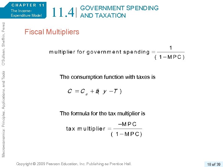
Macroeconomics: Principles, Applications, and Tools O’Sullivan, Sheffrin, Perez 6/e. CHAPTER 11 The Income. Expenditure Model 11. 4 GOVERNMENT SPENDING AND TAXATION Fiscal Multipliers The consumption function with taxes is The formula for the tax multiplier is Copyright © 2009 Pearson Education, Inc. Publishing as Prentice Hall. 18 of 39
Macroeconomics: Principles, Applications, and Tools O’Sullivan, Sheffrin, Perez 6/e. CHAPTER 11 The Income. Expenditure Model 11. 4 GOVERNMENT SPENDING AND TAXATION Using Fiscal Multipliers Though it is very simple, our income-expenditure model illustrates some important lessons: • An increase in government spending will increase total planned expenditures for goods and services. • Cutting taxes will increase the after-tax income of consumers and will also lead to an increase in planned expenditures for goods and services. • Policymakers need to take into account the multipliers for government spending and taxes as they develop policies. In the long run, of course, we are better off if government spends the money wisely, such as on needed infrastructure such as roads and bridges. This is an example of the principle of opportunity cost. P R I N C I P L E O F O P P O RT U N I T Y C O S T The opportunity cost of something is what you sacrifice to get it. Copyright © 2009 Pearson Education, Inc. Publishing as Prentice Hall. 19 of 39

Macroeconomics: Principles, Applications, and Tools O’Sullivan, Sheffrin, Perez 6/e. CHAPTER 11 The Income. Expenditure Model APPLICATION 3 JOHN MAYNARD KEYNES: A WORLD INTELLECTUAL APPLYING THE CONCEPTS #3: How influential a figure was John Maynard Keynes? At King’s College in Cambridge, Keynes began a lifetime association with an important group of writers and artists, the Bloomsbury group, which included the well-regarded writer Virginia Woolf. After World War I, he attended the Versailles Peace Conference and wrote a book, The Economic Consequences of the Peace. • It condemned the peace treaty and its negotiators. • This book established Keynes as both a first-rate economic analyst and a brilliant writer. Between the wars, Keynes wrote his most famous work, The General Theory of Employment, Interest, and Money, which challenged the conventional wisdom that economies would automatically recover from economic downturns. Copyright © 2009 Pearson Education, Inc. Publishing as Prentice Hall. 20 of 39
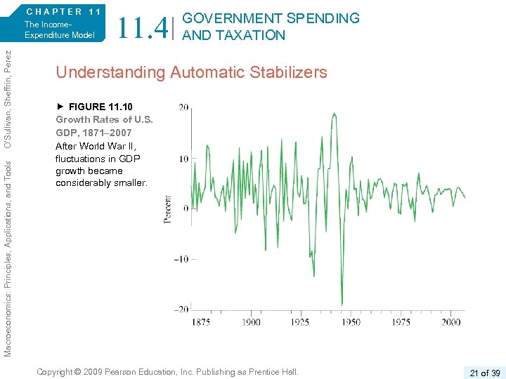
Macroeconomics: Principles, Applications, and Tools O’Sullivan, Sheffrin, Perez 6/e. CHAPTER 11 The Income. Expenditure Model 11. 4 GOVERNMENT SPENDING AND TAXATION Understanding Automatic Stabilizers FIGURE 11. 10 Growth Rates of U. S. GDP, 1871– 2007 After World War II, fluctuations in GDP growth became considerably smaller. Copyright © 2009 Pearson Education, Inc. Publishing as Prentice Hall. 21 of 39
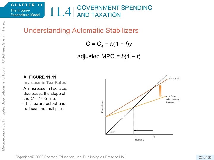
Macroeconomics: Principles, Applications, and Tools O’Sullivan, Sheffrin, Perez 6/e. CHAPTER 11 The Income. Expenditure Model 11. 4 GOVERNMENT SPENDING AND TAXATION Understanding Automatic Stabilizers C = Ca + b(1 − t)y adjusted MPC = b(1 − t) FIGURE 11. 11 Increase in Tax Rates An increase in tax rates decreases the slope of the C + I + G line. This lowers output and reduces the multiplier. Copyright © 2009 Pearson Education, Inc. Publishing as Prentice Hall. 22 of 39
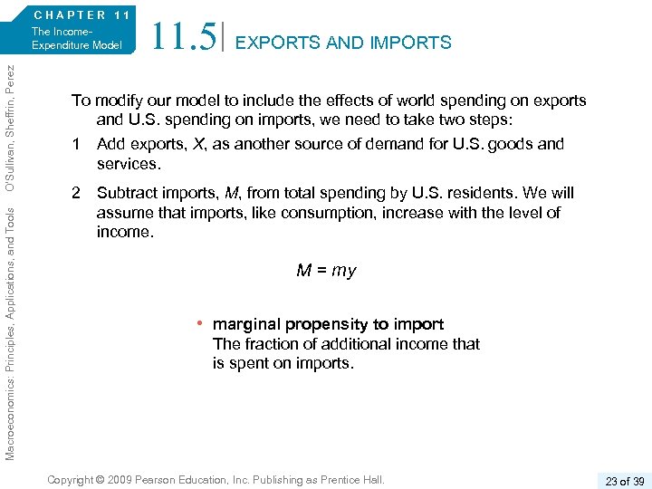
Macroeconomics: Principles, Applications, and Tools O’Sullivan, Sheffrin, Perez 6/e. CHAPTER 11 The Income. Expenditure Model 11. 5 EXPORTS AND IMPORTS To modify our model to include the effects of world spending on exports and U. S. spending on imports, we need to take two steps: 1 Add exports, X, as another source of demand for U. S. goods and services. 2 Subtract imports, M, from total spending by U. S. residents. We will assume that imports, like consumption, increase with the level of income. M = my • marginal propensity to import The fraction of additional income that is spent on imports. Copyright © 2009 Pearson Education, Inc. Publishing as Prentice Hall. 23 of 39
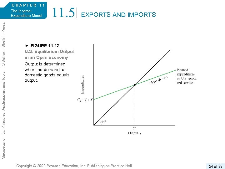
Macroeconomics: Principles, Applications, and Tools O’Sullivan, Sheffrin, Perez 6/e. CHAPTER 11 The Income. Expenditure Model 11. 5 EXPORTS AND IMPORTS FIGURE 11. 12 U. S. Equilibrium Output in an Open Economy Output is determined when the demand for domestic goods equals output. Copyright © 2009 Pearson Education, Inc. Publishing as Prentice Hall. 24 of 39
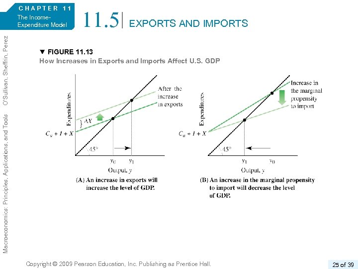
The Income. Expenditure Model 11. 5 EXPORTS AND IMPORTS FIGURE 11. 13 How Increases in Exports and Imports Affect U. S. GDP Macroeconomics: Principles, Applications, and Tools O’Sullivan, Sheffrin, Perez 6/e. CHAPTER 11 Copyright © 2009 Pearson Education, Inc. Publishing as Prentice Hall. 25 of 39
Macroeconomics: Principles, Applications, and Tools O’Sullivan, Sheffrin, Perez 6/e. CHAPTER 11 The Income. Expenditure Model APPLICATION 4 THE LOCOMOTIVE EFFECT: HOW FOREIGN DEMAND AFFECTS A COUNTRY’S OUTPUT APPLYING THE CONCEPTS #4: How do countries benefit from growth in their trading partners? From the early 1990 s until quite recently, the United States was what economists term the “locomotive” for global growth. • Our demand foreign products increased. • U. S. imports increased along with output during this period. • The increased demand fueled exports in foreign countries and promoted their growth. Studies have shown that the increase in demand foreign goods was actually more pronounced for developing countries than for developed countries. Conclusion: The United States was truly a locomotive, pulling the developing countries along. Copyright © 2009 Pearson Education, Inc. Publishing as Prentice Hall. 26 of 39
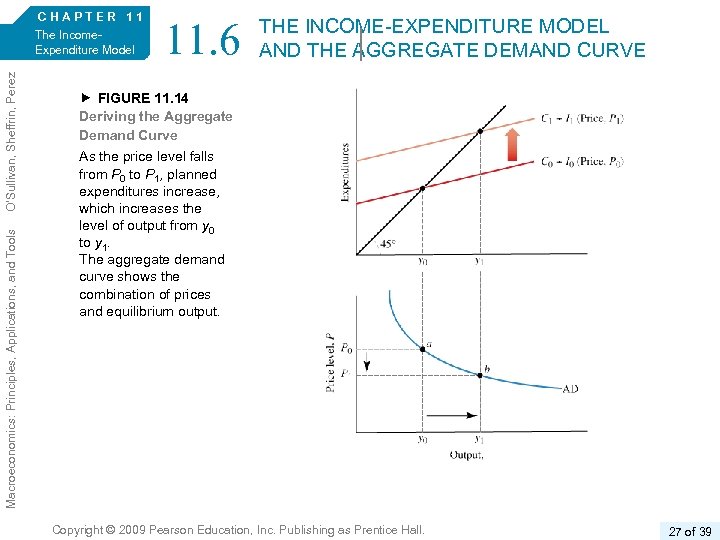
Macroeconomics: Principles, Applications, and Tools O’Sullivan, Sheffrin, Perez 6/e. CHAPTER 11 The Income. Expenditure Model 11. 6 THE INCOME-EXPENDITURE MODEL AND THE AGGREGATE DEMAND CURVE FIGURE 11. 14 Deriving the Aggregate Demand Curve As the price level falls from P 0 to P 1, planned expenditures increase, which increases the level of output from y 0 to y 1. The aggregate demand curve shows the combination of prices and equilibrium output. Copyright © 2009 Pearson Education, Inc. Publishing as Prentice Hall. 27 of 39
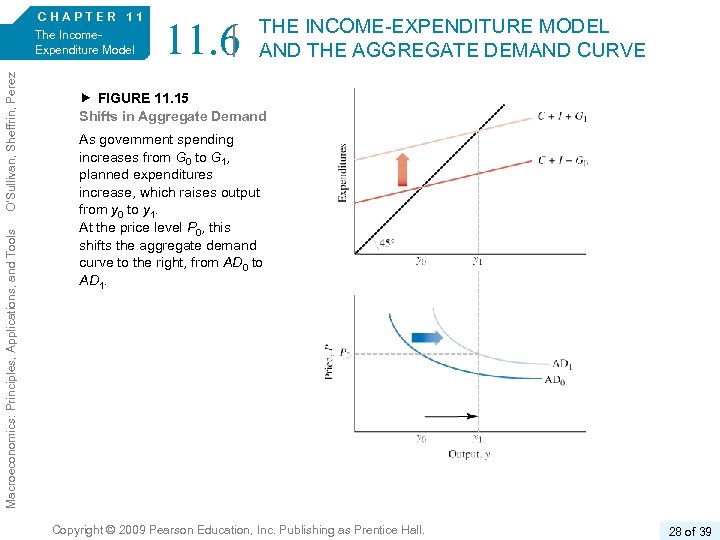
Macroeconomics: Principles, Applications, and Tools O’Sullivan, Sheffrin, Perez 6/e. CHAPTER 11 The Income. Expenditure Model 11. 6 THE INCOME-EXPENDITURE MODEL AND THE AGGREGATE DEMAND CURVE FIGURE 11. 15 Shifts in Aggregate Demand As government spending increases from G 0 to G 1, planned expenditures increase, which raises output from y 0 to y 1. At the price level P 0, this shifts the aggregate demand curve to the right, from AD 0 to AD 1. Copyright © 2009 Pearson Education, Inc. Publishing as Prentice Hall. 28 of 39
Macroeconomics: Principles, Applications, and Tools O’Sullivan, Sheffrin, Perez 6/e. CHAPTER 11 The Income. Expenditure Model KEY TERMS autonomous consumption marginal propensity to consume (MPC) consumption function marginal propensity to import equilibrium output planned expenditures savings function Copyright © 2009 Pearson Education, Inc. Publishing as Prentice Hall. 29 of 39
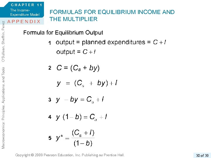
Macroeconomics: Principles, Applications, and Tools O’Sullivan, Sheffrin, Perez 6/e. CHAPTER 11 The Income. Expenditure Model APPENDIX FORMULAS FOR EQUILIBRIUM INCOME AND THE MULTIPLIER Formula for Equilibrium Output 1 2 3 4 5 Copyright © 2009 Pearson Education, Inc. Publishing as Prentice Hall. 30 of 39
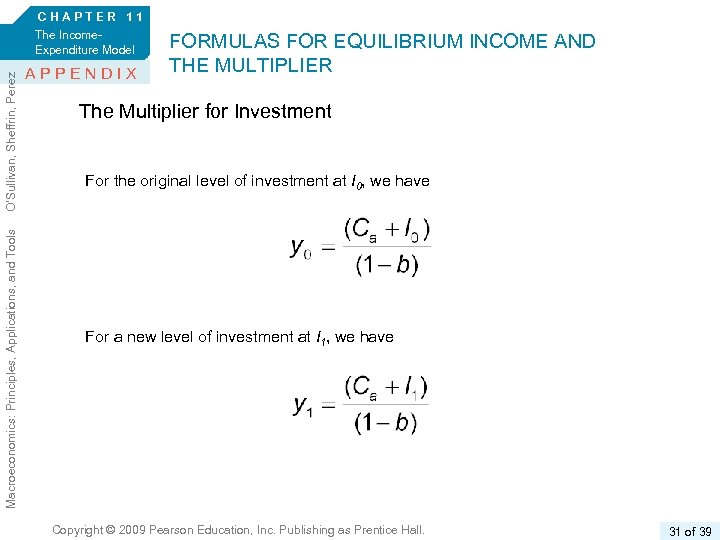
Macroeconomics: Principles, Applications, and Tools O’Sullivan, Sheffrin, Perez 6/e. CHAPTER 11 The Income. Expenditure Model APPENDIX FORMULAS FOR EQUILIBRIUM INCOME AND THE MULTIPLIER The Multiplier for Investment For the original level of investment at I 0, we have For a new level of investment at I 1, we have Copyright © 2009 Pearson Education, Inc. Publishing as Prentice Hall. 31 of 39
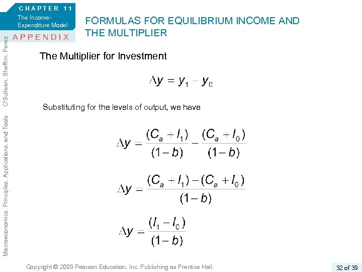
The Income. Expenditure Model APPENDIX FORMULAS FOR EQUILIBRIUM INCOME AND THE MULTIPLIER The Multiplier for Investment Substituting for the levels of output, we have Macroeconomics: Principles, Applications, and Tools O’Sullivan, Sheffrin, Perez 6/e. CHAPTER 11 Copyright © 2009 Pearson Education, Inc. Publishing as Prentice Hall. 32 of 39
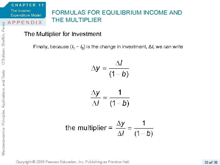
The Income. Expenditure Model APPENDIX FORMULAS FOR EQUILIBRIUM INCOME AND THE MULTIPLIER The Multiplier for Investment Finally, because (I 1 − I 0) is the change in investment, ΔI, we can write Macroeconomics: Principles, Applications, and Tools O’Sullivan, Sheffrin, Perez 6/e. CHAPTER 11 Copyright © 2009 Pearson Education, Inc. Publishing as Prentice Hall. 33 of 39
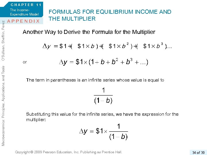
Macroeconomics: Principles, Applications, and Tools O’Sullivan, Sheffrin, Perez 6/e. CHAPTER 11 The Income. Expenditure Model APPENDIX FORMULAS FOR EQUILIBRIUM INCOME AND THE MULTIPLIER Another Way to Derive the Formula for the Multiplier or The term in parentheses is an infinite series whose value is equal to Substituting this value for the infinite series, we have the expression for the multiplier: Copyright © 2009 Pearson Education, Inc. Publishing as Prentice Hall. 34 of 39
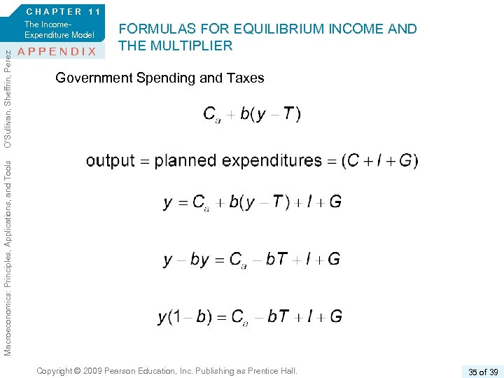
The Income. Expenditure Model APPENDIX FORMULAS FOR EQUILIBRIUM INCOME AND THE MULTIPLIER Government Spending and Taxes Macroeconomics: Principles, Applications, and Tools O’Sullivan, Sheffrin, Perez 6/e. CHAPTER 11 Copyright © 2009 Pearson Education, Inc. Publishing as Prentice Hall. 35 of 39
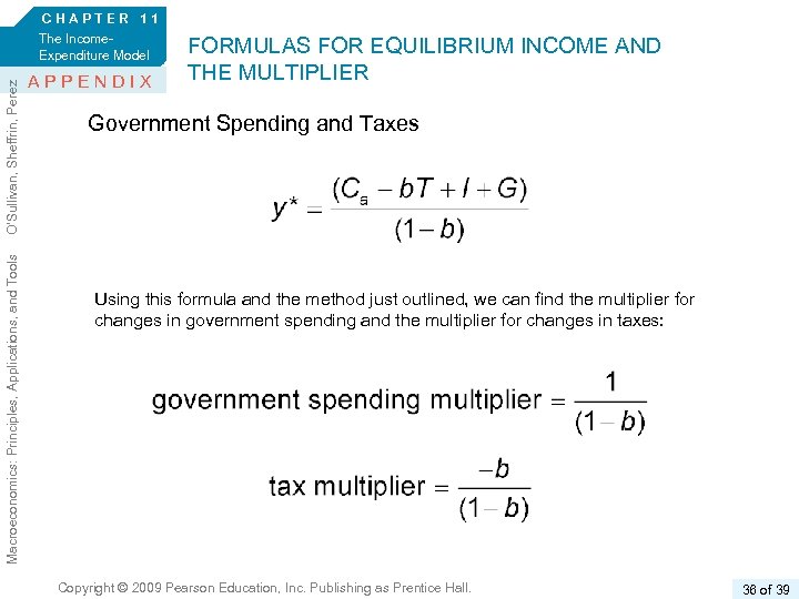
Macroeconomics: Principles, Applications, and Tools O’Sullivan, Sheffrin, Perez 6/e. CHAPTER 11 The Income. Expenditure Model APPENDIX FORMULAS FOR EQUILIBRIUM INCOME AND THE MULTIPLIER Government Spending and Taxes Using this formula and the method just outlined, we can find the multiplier for changes in government spending and the multiplier for changes in taxes: Copyright © 2009 Pearson Education, Inc. Publishing as Prentice Hall. 36 of 39
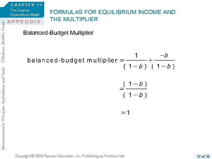
The Income. Expenditure Model APPENDIX FORMULAS FOR EQUILIBRIUM INCOME AND THE MULTIPLIER Balanced-Budget Multiplier Macroeconomics: Principles, Applications, and Tools O’Sullivan, Sheffrin, Perez 6/e. CHAPTER 11 Copyright © 2009 Pearson Education, Inc. Publishing as Prentice Hall. 37 of 39
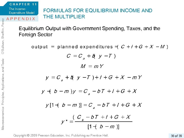
The Income. Expenditure Model APPENDIX FORMULAS FOR EQUILIBRIUM INCOME AND THE MULTIPLIER Equilibrium Output with Government Spending, Taxes, and the Foreign Sector Macroeconomics: Principles, Applications, and Tools O’Sullivan, Sheffrin, Perez 6/e. CHAPTER 11 Copyright © 2009 Pearson Education, Inc. Publishing as Prentice Hall. 38 of 39
b91403eb22c0cebc19973020f116166d.ppt