COORDINATING ECONOMIC ACTIVITY AGGREGATE DEMAND SUPPLY

COORDINATING ECONOMIC ACTIVITY: AGGREGATE DEMAND & SUPPLY

ECONOMIC FLUCTUATIONS • Movements of GDP away from potential output; • Also referred to as business cycles;

KEYNESIAN ECONOMICS • Models based on the idea that demand determines output in the short run; • Short run -- The period of time when prices are fixed;

REAL SHOCKS TO THE ECONOMY One cause of economic fluctuations : • Developing countries dependent on agriculture, which suffer loss to cash crop • Sharp increases in the price of oil can hurt modern economies • Wars can devastate entire regions of the world • Natural disasters can cause sharp reductions in GDP • Major shifts in technology leading to the birth of new industries have profound effects on the economy

REAL BUSINESS CYCLE THEORY • School of economic thought that emphasizes the role that shocks to technology can play in causing economic fluctuations • Led by Edward Prescott of the University of Minnesota • Developed models that integrate technology shocks into classical models • Changes in technology will usually change the level of full employment or potential output • It portrays economic fluctuations as movements in potential output, not as deviations away from potential output

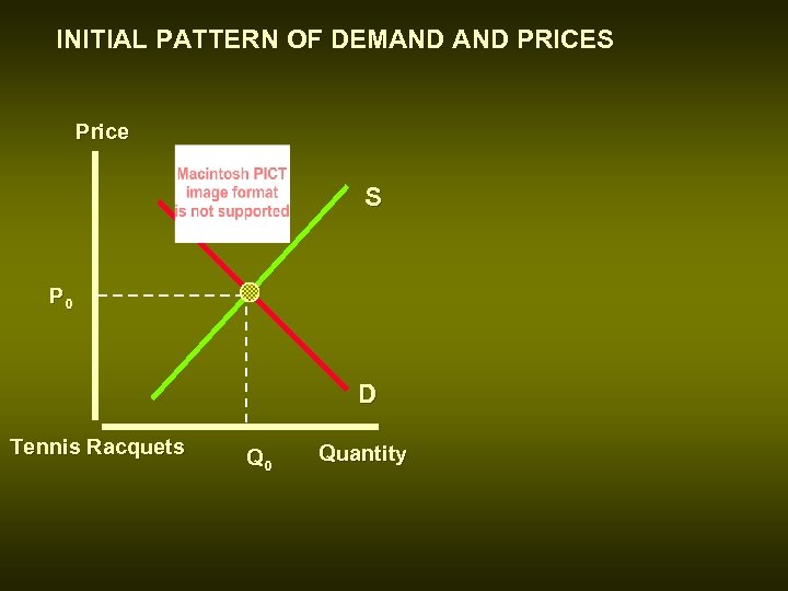INITIAL PATTERN OF DEMAND PRICES Price S P 0 D Tennis Racquets Q 0 Quantity

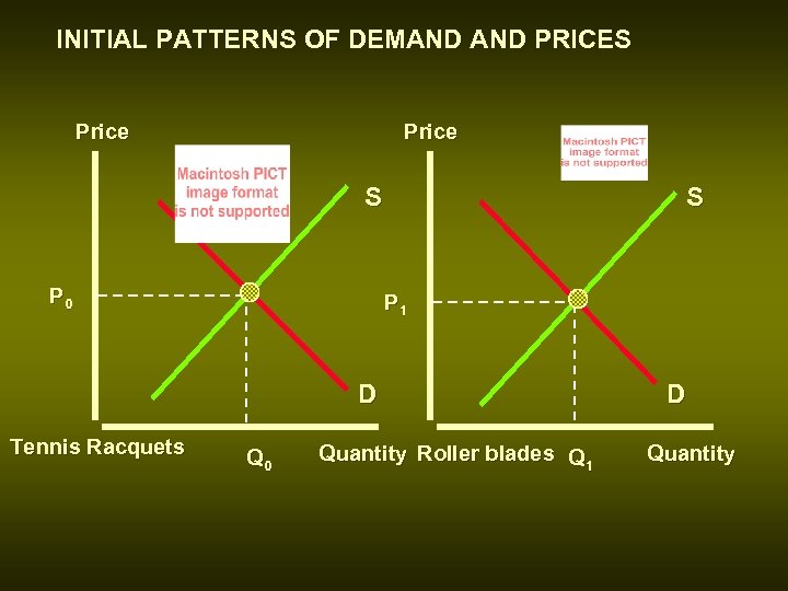INITIAL PATTERNS OF DEMAND PRICES Price S P 0 S P 1 D Tennis Racquets Q 0 Quantity Roller blades Q 1 D Quantity

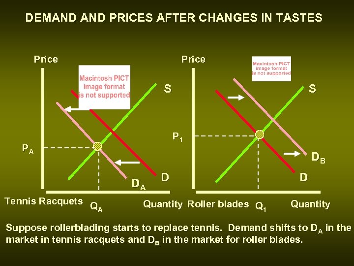DEMAND PRICES AFTER CHANGES IN TASTES Price S P 1 PA DB DA Tennis Racquets Q A S D Quantity Roller blades Q 1 D Quantity Suppose rollerblading starts to replace tennis. Demand shifts to DA in the market in tennis racquets and DB in the market for roller blades.

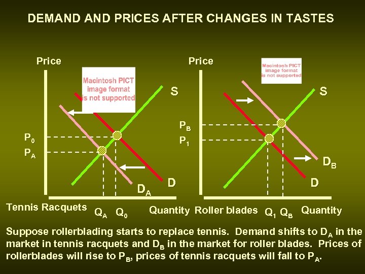DEMAND PRICES AFTER CHANGES IN TASTES Price S PB P 1 P 0 PA DB DA Tennis Racquets Q Q A 0 S D D Quantity Roller blades Q 1 QB Quantity Suppose rollerblading starts to replace tennis. Demand shifts to DA in the market in tennis racquets and DB in the market for roller blades. Prices of rollerblades will rise to PB, prices of tennis racquets will fall to PA.

PRICES AND ECONOMIC COORDINATION • The change in tastes from tennis racquets to rollerblading has caused the economy to produce more roller blades and fewer tennis racquets • The economy accomplishes this through prices • When roller blading became more popular than tennis, the price of roller blades rose and the price of tennis racquets fell • The producers of roller blades were given a signal to step up production • The producers of tennis racquets were given a signal to cut back their production • Workers will leave tennis racquet industry to be employed by roller blade industry

FUTURE PRICES • There is no price for automobiles to be delivered five years from now, so automobiles do not receive any direct signals that consumers wish to purchase automobiles in the future • Only a few commodities, such as metals and certain agricultural commodities, can be traded for future delivery in worldwide markets

TOO LITTLE INFORMATION • Prices may not always contain all the information that producers need • What matters to any firm is the real price: its price relative to all other prices in the economy • Reality Principle: What matters to people is the real value or purchasing power of money or income, not its face value

TOO LITTLE INFORMATION • Problems can occur if firms are uncertain about whether a change in their output price is an increase in the real price or only on the nominal or dollar price • If producers believe demand for their product has fallen, they will cut back production • If this happened throughout the economy, it would lead to a recession

“STICKY” PRICES • If prices are “sticky” or not sufficiently flexible, prices will not coordinate activity as efficiently • In modern economies, some prices are flexible, while others are not • Auction Prices -- those determined on nearly a daily basis • Prices for fresh fish, vegetables, and other food are very flexible • Custom Prices -- those that adjust rather slowly • Prices for industrial commodities, such as steel rods or machine tools, are custom prices

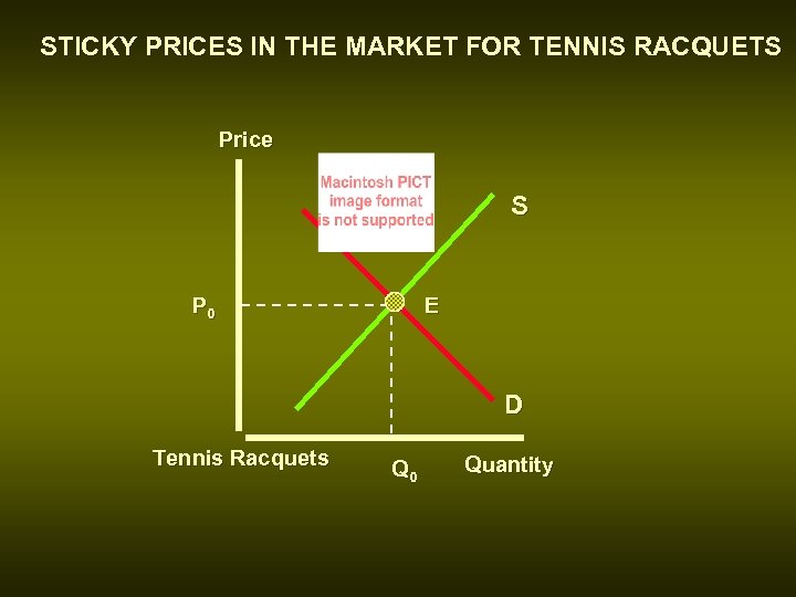STICKY PRICES IN THE MARKET FOR TENNIS RACQUETS Price S P 0 E D Tennis Racquets Q 0 Quantity

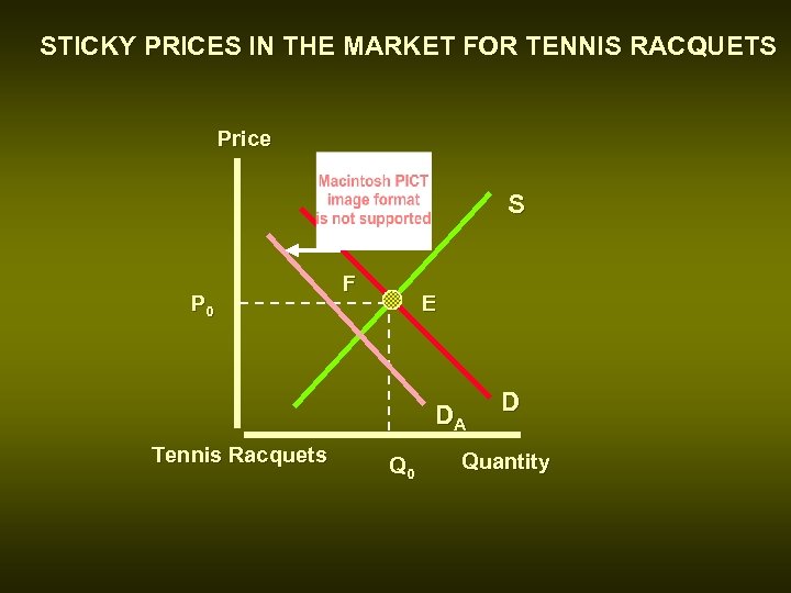STICKY PRICES IN THE MARKET FOR TENNIS RACQUETS Price S P 0 F E DA Tennis Racquets Q 0 D Quantity

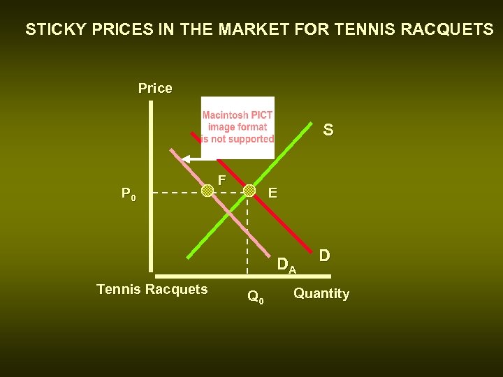STICKY PRICES IN THE MARKET FOR TENNIS RACQUETS Price S P 0 F E DA Tennis Racquets Q 0 D Quantity

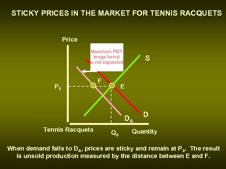STICKY PRICES IN THE MARKET FOR TENNIS RACQUETS Price S P 0 F E DA Tennis Racquets Q 0 D Quantity When demand falls to DA, prices are sticky and remain at P 0. The result is unsold production measured by the distance between E and F.

WAGES • Wages, the price of labor, adjust extremely slowly • Workers often have long-term contracts that do not allow wages to change at all during a given year • Even unskilled, low-wage workers are often protected from decreases in their wages by minimum wage laws • For most firms, wages are the single most important cost of doing business • If wages are sticky, their overall costs will be sticky • Stickiness of wages reinforces stickiness of prices

SHORT-RUN PRICES ARE STICKY • Firms let demand determine level of output in the short run • Automaker may have higher demand if autos are popular or lower demand if autos are unpopular • Steelmaker who provides steel to automaker may provide more or less steel without adjusting price • The same principle applies to workers • During good times a company will employ many workers and may even require some to work overtime with no wage change • The short run in macroeconomics is the period when prices are fixed

LONG-RUN PRICES • In the long run, price adjust fully to changes in demand • Over short periods of time, the presence of formal and informal contracts mean that demand will be reflected primarily in changes in output, not prices

AGGREGATE DEMAND • The aggregate demand curve plots the total demand for GDP as a function of price level • The aggregate demand curve is downward sloping • As the price level falls, the total demand for goods and services increases

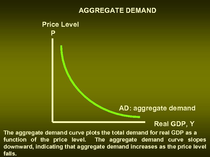AGGREGATE DEMAND Price Level P AD: aggregate demand Real GDP, Y The aggregate demand curve plots the total demand for real GDP as a function of the price level. The aggregate demand curve slopes downward, indicating that aggregate demand increases as the price level falls.

REALITY PRINCIPLE What matters to people is the real value or purchasing power of money or income, not its face value.

WEALTH EFFECT • Increase in spending that occurs because the real value of money increases when the price level falls • One of the key reasons that aggregate demand slopes downward

TWO OTHER REASONS WHY DEMAND CURVE SLOPES DOWNWARD • Interest rate effect With a given supply of money in the economy, a lower price level will lead to lower interest rates As interest rates fall, demand for investment goods in the economy increase. • Effects from international trade In an open economy, a lower price level will mean that domestic goods become cheaper relative to foreign goods and demand for domestic goods will increase

SHIFTS OF AGGREGATE DEMAND • At any price level, an increase in aggregate demand means that total demand for real GDP has increased, and the curve shifts to the right • Factors that decrease the aggregate demand will shift the aggregate demand curve to the left • At any price level, a decrease in aggregate demand means that total demand for real GDP has decreased

KEY FACTORS THAT SHIFT THE AGGREGATE DEMAND CURVE • Changes in the supply of money • Changes in taxes • Changes in government spending • other factors

CHANGES IN THE SUPPLY OF MONEY • An increase in the supply of money in the economy will increase aggregate demand shift the demand curve right • At any price level, a higher supply of money will mean more consumer wealth and an increased demand for goods and services • A decrease in the supply of money will decrease aggregate demand shift the aggregate demand curve to the left

CHANGES IN TAXES • A decrease in taxes will increase aggregate demand shift the aggregate demand curve to the right • Lower taxes will increase income available to households and increase their spending on goods and services • Increases in taxes will decrease the aggregate demand shift the aggregate demand curve left

CHANGES IN GOVERNMENT SPENDING • An increase in government spending will increase aggregate demand shift the aggregate demand curve right • Since the government is a source of demand for goods and services, higher government spending naturally leads to an increase in total demand for goods and services • Decreases in government spending will decrease aggregate demand shift the curve to the left

OTHER FACTORS • Any change in demand from households, firms, or the foreign sector will also change aggregate demand • When shifts in aggregate demand are discussed, any changes that arise from movements in the price level are not to be included

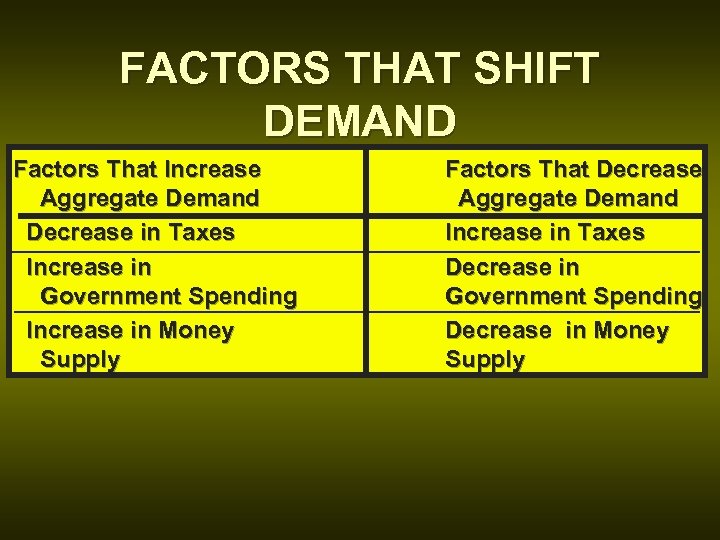FACTORS THAT SHIFT DEMAND Factors That Increase Aggregate Demand Decrease in Taxes Increase in Government Spending Increase in Money Supply Factors That Decrease Aggregate Demand Increase in Taxes Decrease in Government Spending Decrease in Money Supply

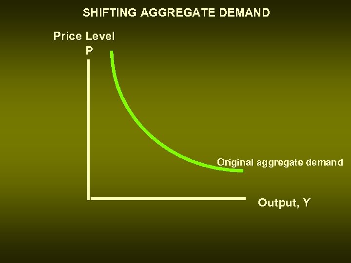SHIFTING AGGREGATE DEMAND Price Level P Original aggregate demand Output, Y

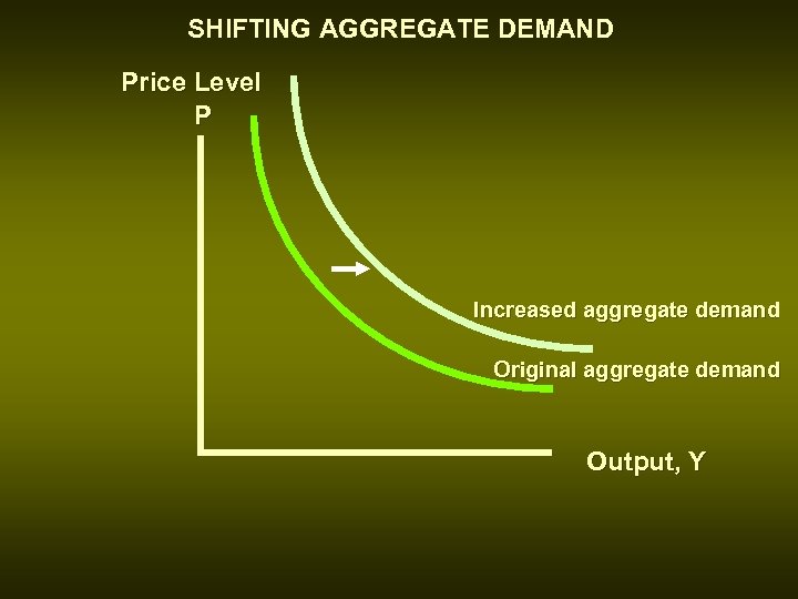SHIFTING AGGREGATE DEMAND Price Level P Increased aggregate demand Original aggregate demand Output, Y

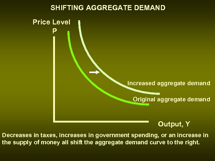SHIFTING AGGREGATE DEMAND Price Level P Increased aggregate demand Original aggregate demand Output, Y Decreases in taxes, increases in government spending, or an increase in the supply of money all shift the aggregate demand curve to the right.

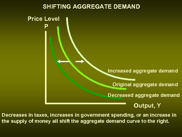SHIFTING AGGREGATE DEMAND Price Level P Increased aggregate demand Original aggregate demand Decreased aggregate demand Output, Y Decreases in taxes, increases in government spending, or an increase in the supply of money all shift the aggregate demand curve to the right.

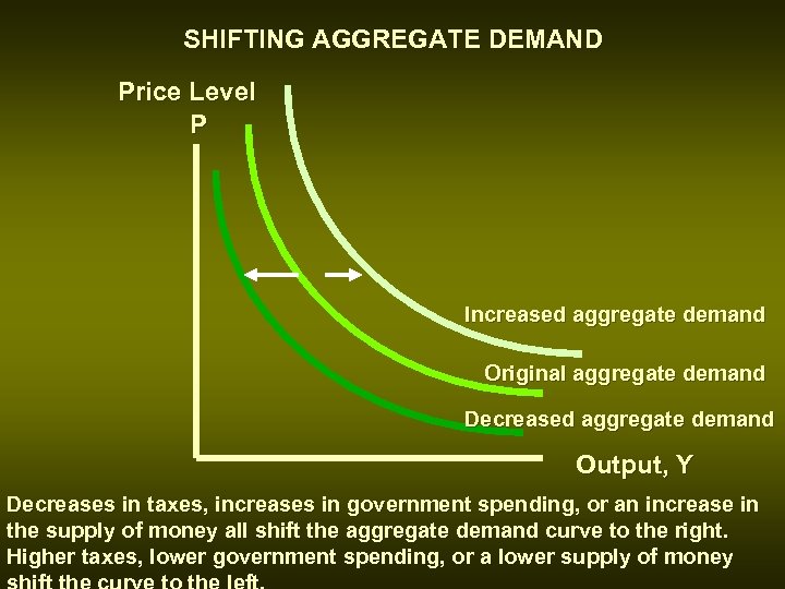SHIFTING AGGREGATE DEMAND Price Level P Increased aggregate demand Original aggregate demand Decreased aggregate demand Output, Y Decreases in taxes, increases in government spending, or an increase in the supply of money all shift the aggregate demand curve to the right. Higher taxes, lower government spending, or a lower supply of money

AGGREGATE SUPPLY • Depicts the relationship between the level of prices and real GDP • Two different aggregate supply curves, which correspond to the long run and the short run: -- classical aggregate supply curve -- Keynesian aggregate supply curve

CLASSICAL AGGREGATE SUPPLY CURVE • Aggregate supply curve for the long run when the economy is at full employment • Full-employment output depends solely on the supply of capital and labor and the state of technology • full-employment output does not depend on the price level • Classical aggregate supply curve is plotted as a vertical line (unaffected by prices)

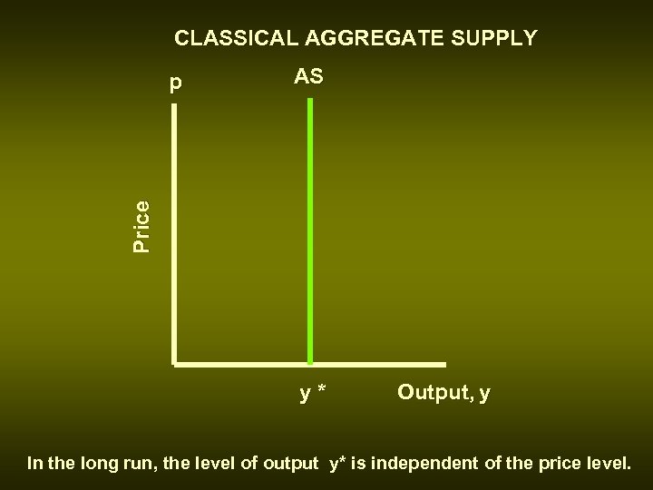CLASSICAL AGGREGATE SUPPLY AS Price p y* Output, y In the long run, the level of output y* is independent of the price level.

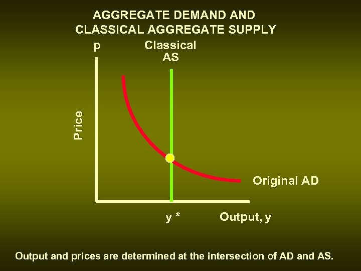Price AGGREGATE DEMAND CLASSICAL AGGREGATE SUPPLY p Classical AS Original AD y* Output, y Output and prices are determined at the intersection of AD and AS.

COMBINING AGGREGATE DEMAND AGGREGATE SUPPLY • The price level and level of output are determined by the intersection of aggregate supply and aggregate demand • At that point, total amount demanded will just equal the total amount supplied • The position of the aggregate demand curve will depend on the level of taxes, government spending, and the supply of money • The full-employment output determines the classical aggregate supply curve

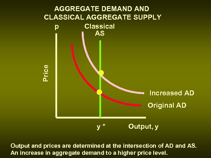Price AGGREGATE DEMAND CLASSICAL AGGREGATE SUPPLY p Classical AS Increased AD Original AD y* Output, y Output and prices are determined at the intersection of AD and AS. An increase in aggregate demand to a higher price level.

COMBINING AGGREGATE DEMAND AGGREGATE SUPPLY • An increase in demand will shift the aggregate demand curve right • With a classical aggregate supply curve, the increase in aggregate demand will raise the prices but leave the level of output unchanged

THE KEYNESIAN AGGREGATE SUPPLY CURVE • The Keynesian aggregate supply curve is horizontal in the short run • Firms are assumed to supply all output that is demanded at the current price • Formal and informal contracts commit producers to supply all that is demanded at the going price • The entire Keynesian supply curve can shift up or down as prices adjust to their longrun levels

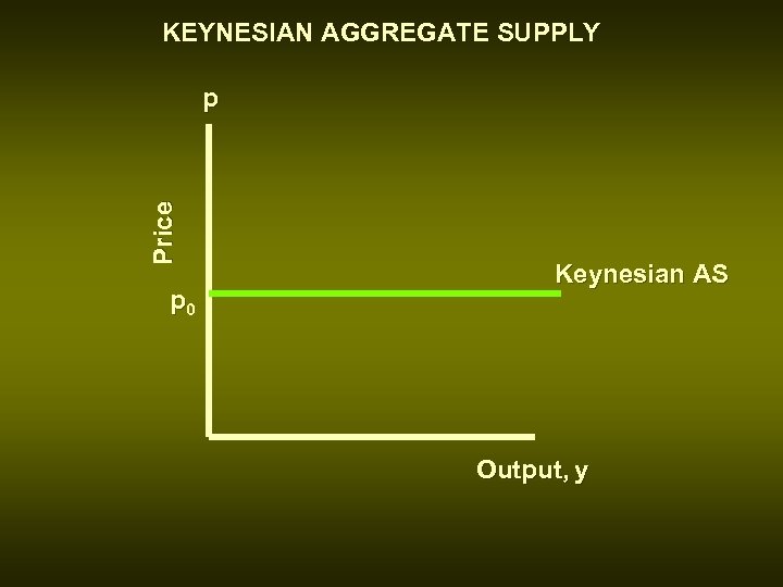KEYNESIAN AGGREGATE SUPPLY Price p p 0 Keynesian AS Output, y

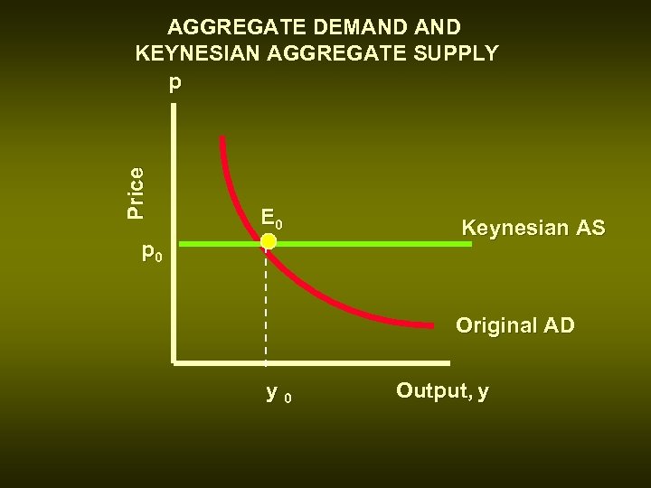Price AGGREGATE DEMAND KEYNESIAN AGGREGATE SUPPLY p E 0 p 0 Keynesian AS Original AD y 0 Output, y

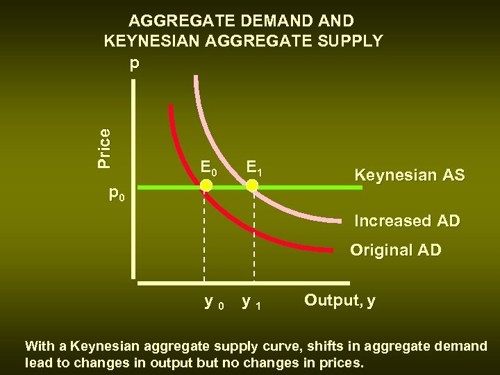Price AGGREGATE DEMAND KEYNESIAN AGGREGATE SUPPLY p E 0 E 1 p 0 Keynesian AS Increased AD Original AD y 0 y 1 Output, y With a Keynesian aggregate supply curve, shifts in aggregate demand lead to changes in output but no changes in prices.

AGGREGATE DEMAND KEYNESIAN AGGREGATE SUPPLY CURVES • The intersection of AD and AS curves determines the price level and the level of output at point E • Since aggregate demand is horizontal, aggregate demand totally determines the level of output • As aggregate demand increases, the new equilibrium will be at the same price p 0, but output will increase from y 0 to y 1 • The Keynesian aggregate supply curve need not correspond to full-employment output • Changes in demand will lead to economic fluctuations with sticky prices and a Keynesian aggregate supply curve

SUPPLY SHOCKS • External disturbances that shift the aggregate supply curve • Most important illustrations of supply shocks for the world economy have been sharp increases in the price of oil that occurred in 1973 and 1979 – When oil prices increased sharply, firms would no longer sell all the goods and services that were demanded at the current price – To maintain their profit levels, firms raised their prices

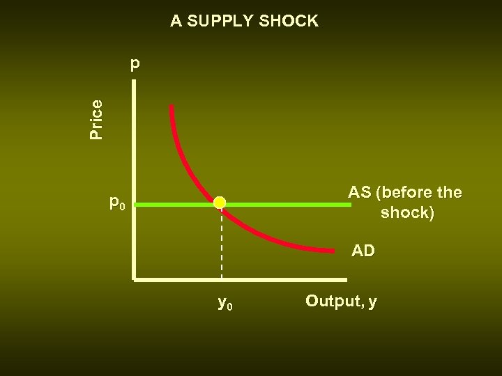A SUPPLY SHOCK Price p AS (before the shock) p 0 AD y 0 Output, y

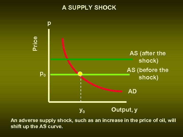A SUPPLY SHOCK Price p AS (after the shock) AS (before the shock) p 0 AD y 0 Output, y An adverse supply shock, such as an increase in the price of oil, will shift up the AS curve.

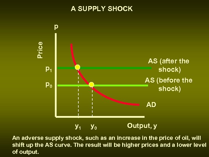A SUPPLY SHOCK Price p p 1 AS (after the shock) p 0 AS (before the shock) AD y 1 y 0 Output, y An adverse supply shock, such as an increase in the price of oil, will shift up the AS curve. The result will be higher prices and a lower level of output.

LINKS BETWEEN SHORT RUN AND LONG RUN • Provided by adjustments of wages and prices -- sticky and do not move immediately in the short run -- Over time adjust and the economy reaches its long-run equilibrium • Wage and price adjustments provide the links between Keynesian and classical economics

WAGES AND PRICES IN AN ECONOMY PRODUCING AT A LEVEL ABOVE FULL EMPLOYMENT • • The Wage Price Spiral Firms find it increasingly difficult to hire and retain workers Workers find it easy to obtain a job and easy to change jobs To attract workers and to prevent others from quitting, firms raise their wages to try to outbid their competitors The actions of firms start a process in which wages increase throughout the economy

PRICES IN AN ECONOMY PRODUCING AT A LEVEL ABOVE FULL EMPLOYMENT • • • The Wage Price Spiral For most firms, wages are the largest single cost of production As their labor costs increase, firms have no choice but to increase prices as well As prices rise, workers know they need higher dollar or nominal wages to maintain their real wage The Reality Principle What matters to people is the real value or purchasing power of money or income, not its face value

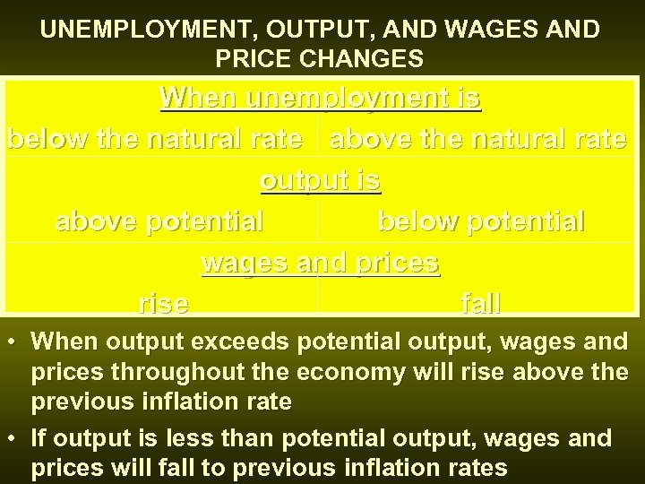UNEMPLOYMENT, OUTPUT, AND WAGES AND PRICE CHANGES When unemployment is below the natural rate above the natural rate output is above potential below potential wages and prices rise fall • When output exceeds potential output, wages and prices throughout the economy will rise above the previous inflation rate • If output is less than potential output, wages and prices will fall to previous inflation rates

AGGREGATE DEMAND • The aggregate demand curve is plotted with the price on the vertical axis and real output on the horizontal axis • It shows the total level of demand for goods and services for any level of output

AGGREGATE SUPPLY • The classical aggregate supply curve (long run) is a vertical line at the full-employment level of output • The Keynesian aggregate supply curve (short run) is a horizontal line at the current level of prices • The Keynesian aggregate supply curve is horizontal because changes in demand lead to very small changes in prices over short periods of time

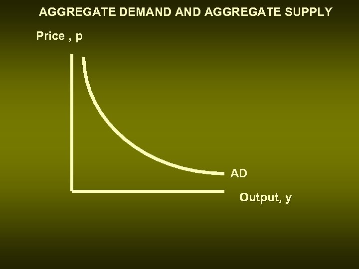AGGREGATE DEMAND AGGREGATE SUPPLY Price , p AD Output, y

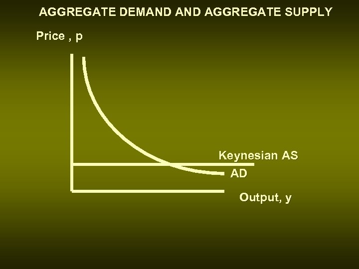AGGREGATE DEMAND AGGREGATE SUPPLY Price , p Keynesian AS AD Output, y

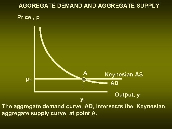AGGREGATE DEMAND AGGREGATE SUPPLY Price , p p 0 A Keynesian AS AD Output, y y 0 The aggregate demand curve, AD, intersects the Keynesian aggregate supply curve at point A.

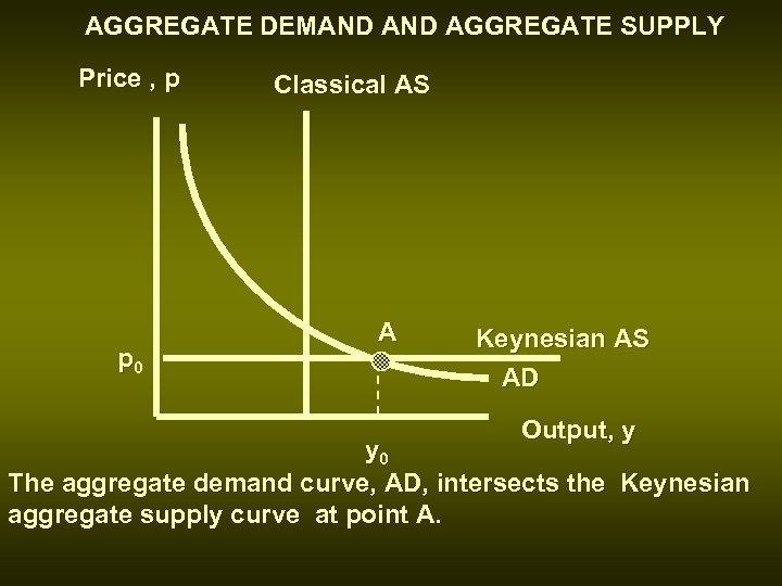AGGREGATE DEMAND AGGREGATE SUPPLY Price , p p 0 Classical AS A Keynesian AS AD Output, y y 0 The aggregate demand curve, AD, intersects the Keynesian aggregate supply curve at point A.

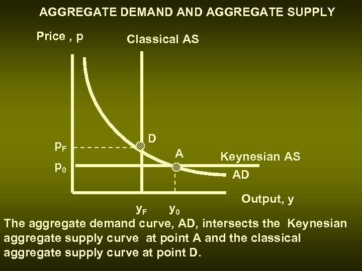AGGREGATE DEMAND AGGREGATE SUPPLY Price , p p. F p 0 Classical AS D A Keynesian AS AD Output, y y. F y 0 The aggregate demand curve, AD, intersects the Keynesian aggregate supply curve at point A and the classical aggregate supply curve at point D.

RELATING KEYNESIAN TO CLASSICAL POSITIONS • At the intersection of aggregate demand Keynesian aggregate supply curves, the current level of output Y 0, exceeds the full-employment level of output, YF • Unemployment rate is below the natural rate • Firms find it difficult to hire and retain workers, and wage-price spiral begins • As level of prices increase, Keynesian aggregate supply curve shifts up over time • The shift in the Keynesian aggregate supply curve will bring the economy to long-run equilibrium -- the intersection of classical AS and AD

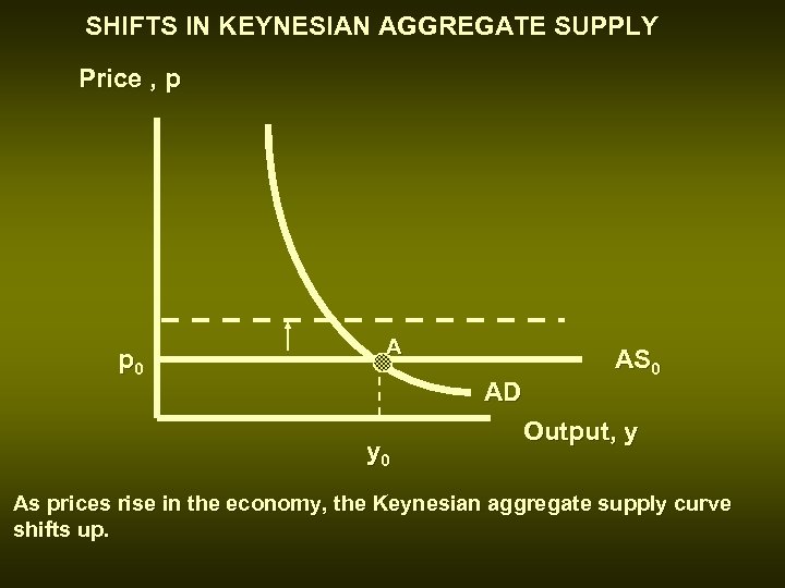SHIFTS IN KEYNESIAN AGGREGATE SUPPLY Price , p p 0 A AD y 0 AS 0 Output, y As prices rise in the economy, the Keynesian aggregate supply curve shifts up.

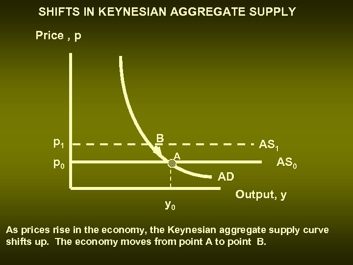SHIFTS IN KEYNESIAN AGGREGATE SUPPLY Price , p p 1 p 0 B A AD y 0 AS 1 AS 0 Output, y As prices rise in the economy, the Keynesian aggregate supply curve shifts up. The economy moves from point A to point B.

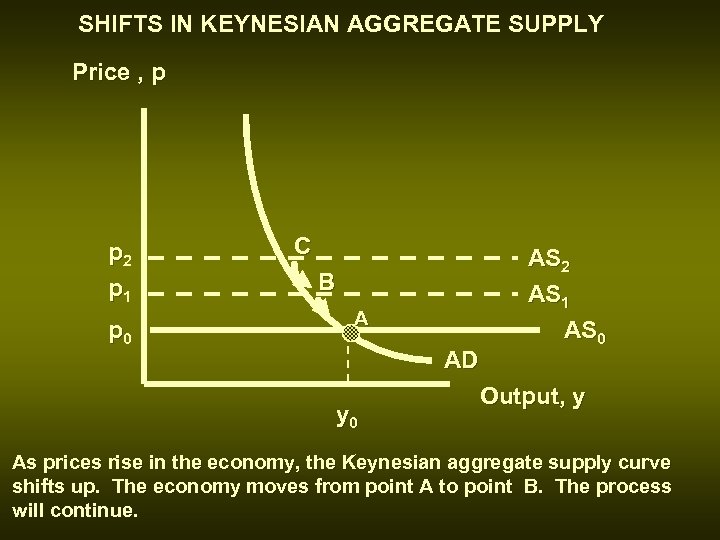SHIFTS IN KEYNESIAN AGGREGATE SUPPLY Price , p p 2 p 1 p 0 C B A AD y 0 AS 2 AS 1 AS 0 Output, y As prices rise in the economy, the Keynesian aggregate supply curve shifts up. The economy moves from point A to point B. The process will continue.

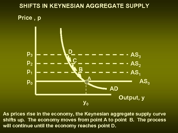SHIFTS IN KEYNESIAN AGGREGATE SUPPLY Price , p p 3 p 2 p 1 p 0 D C B A AD y 0 AS 3 AS 2 AS 1 AS 0 Output, y As prices rise in the economy, the Keynesian aggregate supply curve shifts up. The economy moves from point A to point B. The process will continue until the economy reaches point D.

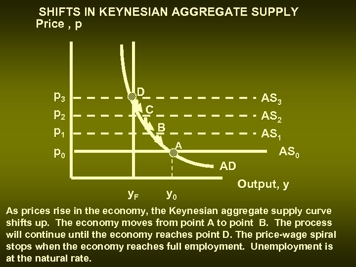SHIFTS IN KEYNESIAN AGGREGATE SUPPLY Price , p p 3 p 2 p 1 D C B A p 0 AD y. F y 0 AS 3 AS 2 AS 1 AS 0 Output, y As prices rise in the economy, the Keynesian aggregate supply curve shifts up. The economy moves from point A to point B. The process will continue until the economy reaches point D. The price-wage spiral stops when the economy reaches full employment. Unemployment is at the natural rate.

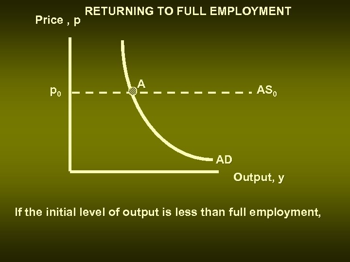Price , p p 0 RETURNING TO FULL EMPLOYMENT A AS 0 AD Output, y If the initial level of output is less than full employment,

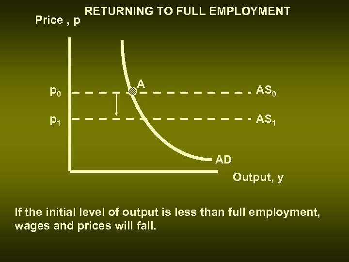Price , p p 0 RETURNING TO FULL EMPLOYMENT A AS 0 p 1 AS 1 AD Output, y If the initial level of output is less than full employment, wages and prices will fall.

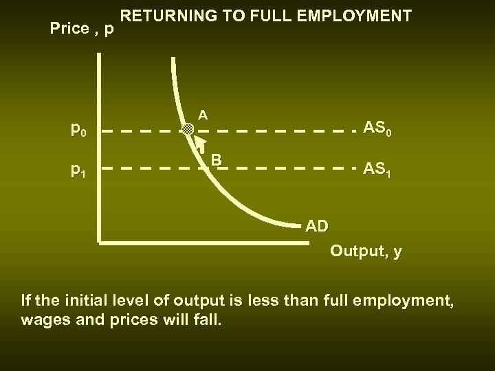Price , p p 0 p 1 RETURNING TO FULL EMPLOYMENT A AS 0 B AS 1 AD Output, y If the initial level of output is less than full employment, wages and prices will fall.

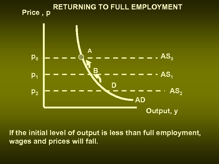Price , p p 0 p 1 p 2 RETURNING TO FULL EMPLOYMENT A AS 0 B AS 1 D AD AS 2 Output, y If the initial level of output is less than full employment, wages and prices will fall.

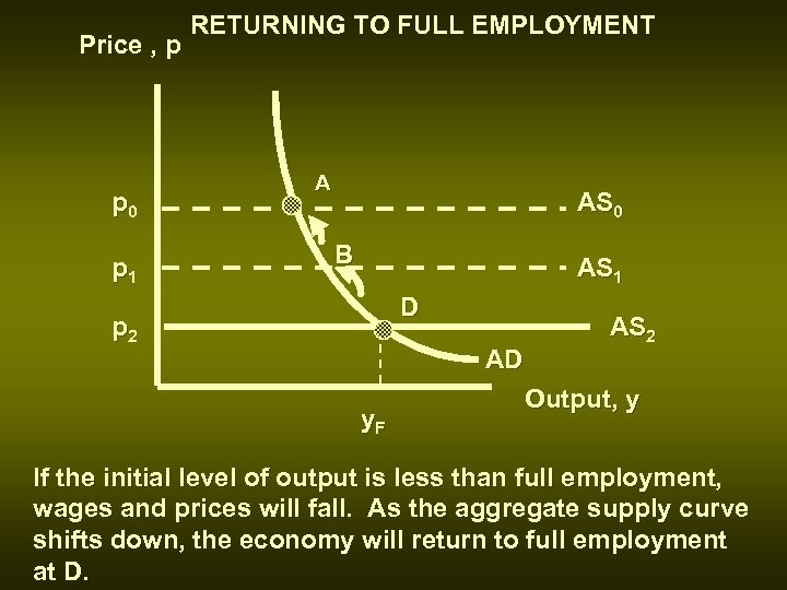Price , p p 0 p 1 RETURNING TO FULL EMPLOYMENT A AS 0 B AS 1 D p 2 AD y. F AS 2 Output, y If the initial level of output is less than full employment, wages and prices will fall. As the aggregate supply curve shifts down, the economy will return to full employment at D.

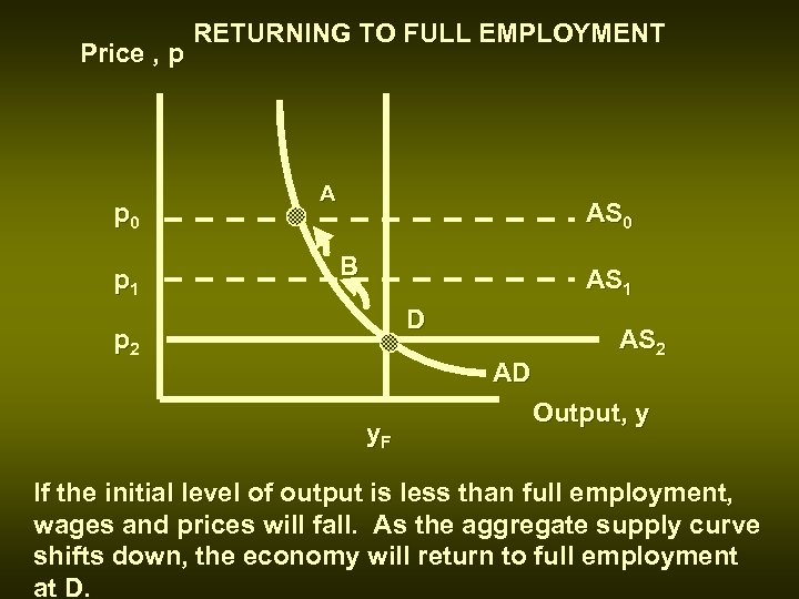Price , p p 0 p 1 RETURNING TO FULL EMPLOYMENT A AS 0 B AS 1 D p 2 AD y. F AS 2 Output, y If the initial level of output is less than full employment, wages and prices will fall. As the aggregate supply curve shifts down, the economy will return to full employment at D.

THE ECONOMY WILL EVENTUALLY RETURN TO FULL EMPLOYMENT • If output exceeds full employment, prices will rise and output will fall back to full employment • If output is less than full employment, prices will fall as the economy returns to full employment

MOVING FROM THE SHORT TO THE LONG RUN • Economists disagree about the time it takes: range between 2 and 6 years • Alternatives bring long-run (full employment) about -- Do nothing and allow adjustment process, with falling wages and prices to return the economy to full employment -- Use expansionary policies (open market purchases, increases in government spending or tax cuts) to shift the aggregate demand curve right -- Use contractionary policies to reduce demand / level of GDP until it reaches potential output

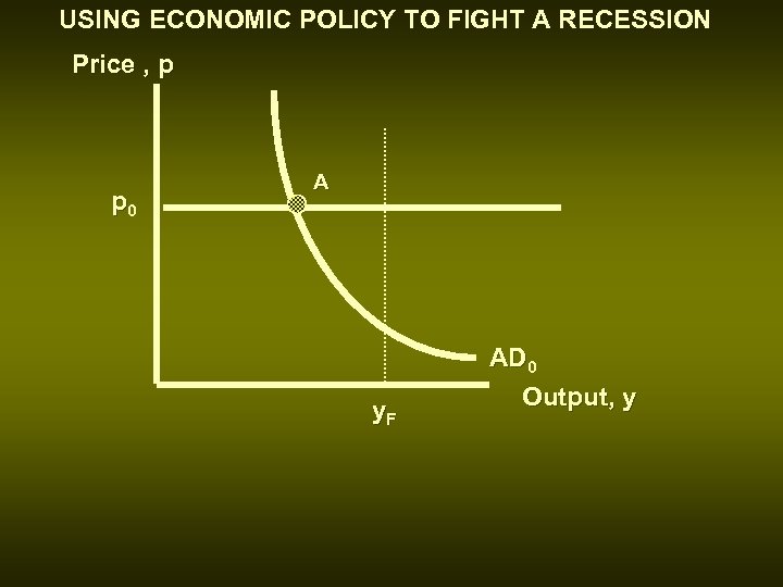USING ECONOMIC POLICY TO FIGHT A RECESSION Price , p p 0 A y. F AD 0 Output, y

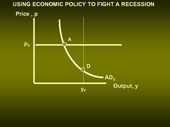USING ECONOMIC POLICY TO FIGHT A RECESSION Price , p p 0 A D y. F AD 0 Output, y

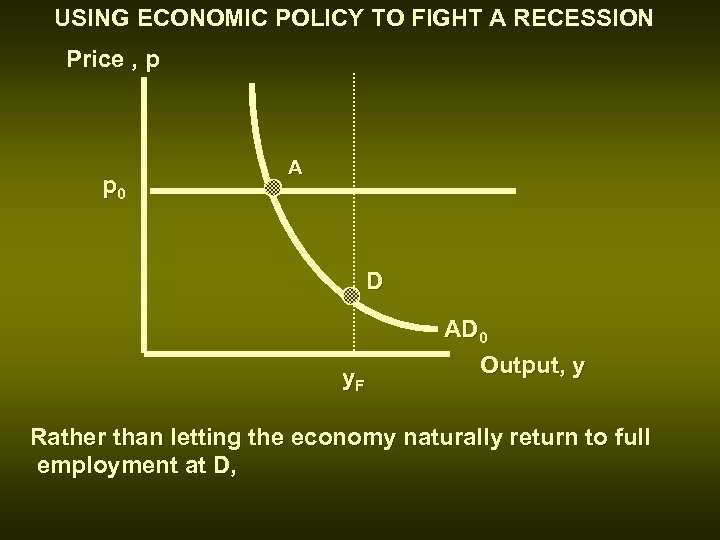USING ECONOMIC POLICY TO FIGHT A RECESSION Price , p p 0 A D y. F AD 0 Output, y Rather than letting the economy naturally return to full employment at D,

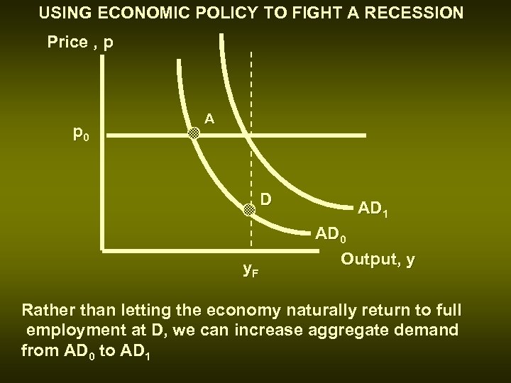USING ECONOMIC POLICY TO FIGHT A RECESSION Price , p p 0 A D y. F AD 1 AD 0 Output, y Rather than letting the economy naturally return to full employment at D, we can increase aggregate demand from AD 0 to AD 1

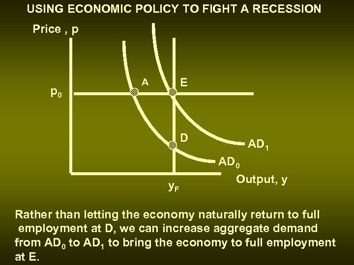USING ECONOMIC POLICY TO FIGHT A RECESSION Price , p p 0 E A D y. F AD 1 AD 0 Output, y Rather than letting the economy naturally return to full employment at D, we can increase aggregate demand from AD 0 to AD 1 to bring the economy to full employment at E.

ACTIVE ECONOMIC POLICIES AND ECONOMIC STABILITY • Active economic policies are more likely to destabilize the economy if the adjustment process operates quickly • Economists who believe the economy adjusts rapidly to full employment generally oppose using monetary or fiscal policy to try to stabilize the economy • Economists who believe the adjustment process operates slowly are more sympathetic to using monetary or fiscal policy to stabilize the economy • It is possible for the speed of adjustment to vary over time, making decisions about policy more difficult

THE ADJUSTMENT PROCESS • Interest rates are determined by the demand supply of money • Interest rates determine the level of investment spending in the economy • Investment spending, along with consumption, government spending and net exports determines the level of GDP

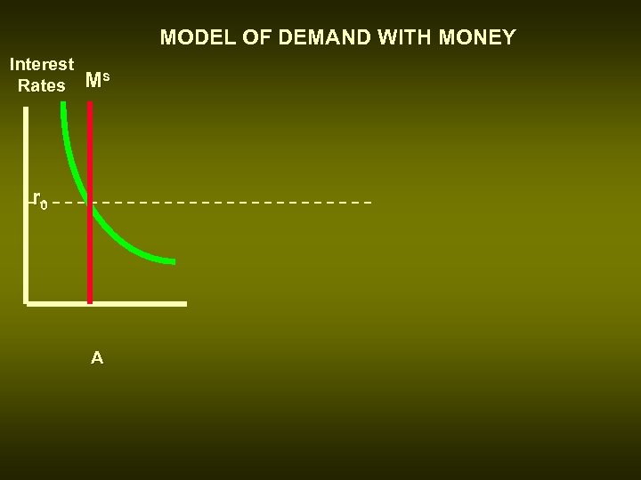MODEL OF DEMAND WITH MONEY Interest Rates Ms r 0 A

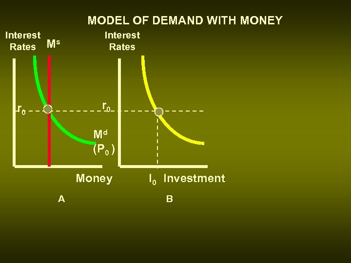MODEL OF DEMAND WITH MONEY Interest Rates Ms Interest Rates r 0 Md (P 0 ) Money A I 0 Investment B

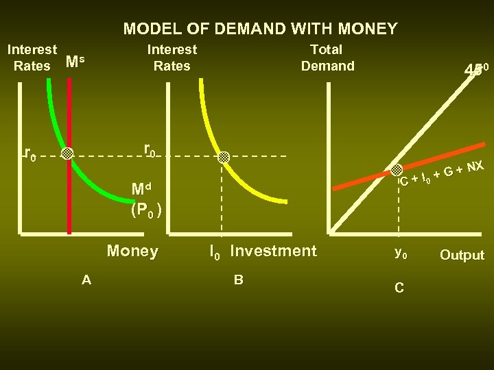MODEL OF DEMAND WITH MONEY Interest Rates Ms Interest Rates Total Demand 450 r 0 C Md (P 0 ) Money A I 0 Investment B y 0 C + I 0 + G + NX Output

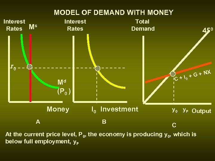MODEL OF DEMAND WITH MONEY Interest Rates Ms Interest Rates Total Demand 450 r 0 C Md (P 0 ) Money A I 0 Investment B + I 0 + G + NX y 0 y. F Output C At the current price level, P 0, the economy is producing y 0, which is below full employment, y. F

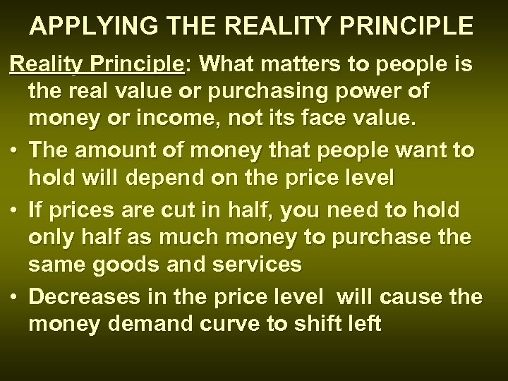APPLYING THE REALITY PRINCIPLE Reality Principle: What matters to people is the real value or purchasing power of money or income, not its face value. • The amount of money that people want to hold will depend on the price level • If prices are cut in half, you need to hold only half as much money to purchase the same goods and services • Decreases in the price level will cause the money demand curve to shift left

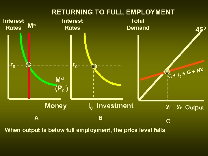RETURNING TO FULL EMPLOYMENT Interest Rates Ms Interest Rates r 0 Total Demand 450 r 0 C Md (P 0 ) Money A I 0 Investment B When output is below full employment, the price level falls + I 0 + G + NX y 0 y. F Output C

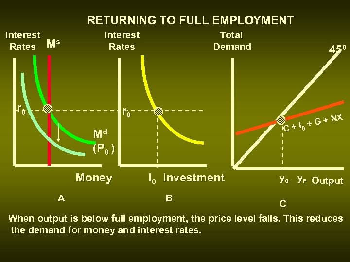RETURNING TO FULL EMPLOYMENT Interest Rates Ms Interest Rates r 0 Total Demand 450 r 0 C Md (P 0 ) Money A I 0 Investment B + I 0 + G + NX y 0 y. F Output C When output is below full employment, the price level falls. This reduces the demand for money and interest rates.

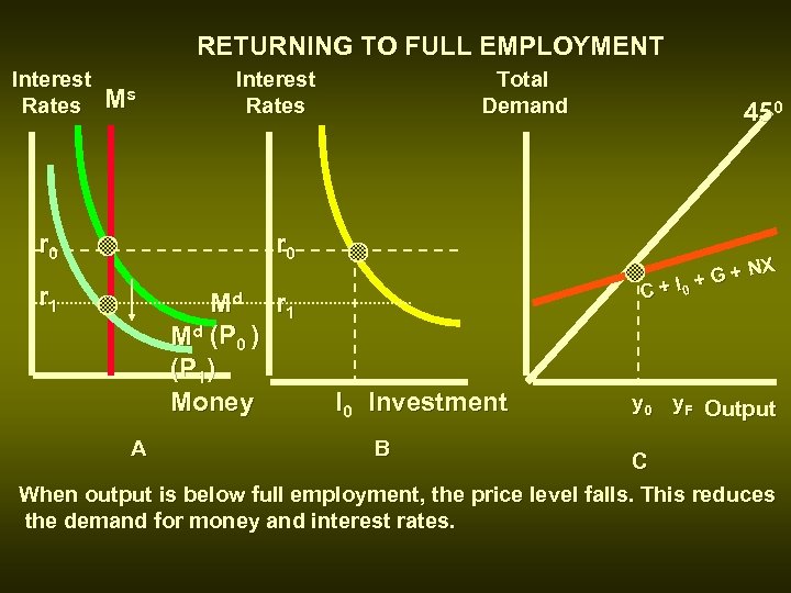RETURNING TO FULL EMPLOYMENT Interest Rates Ms Interest Rates r 0 Md r 1 Md (P 0 ) (P 1) Money 450 r 1 Total Demand A C I 0 Investment B + I 0 + G + NX y 0 y. F Output C When output is below full employment, the price level falls. This reduces the demand for money and interest rates.

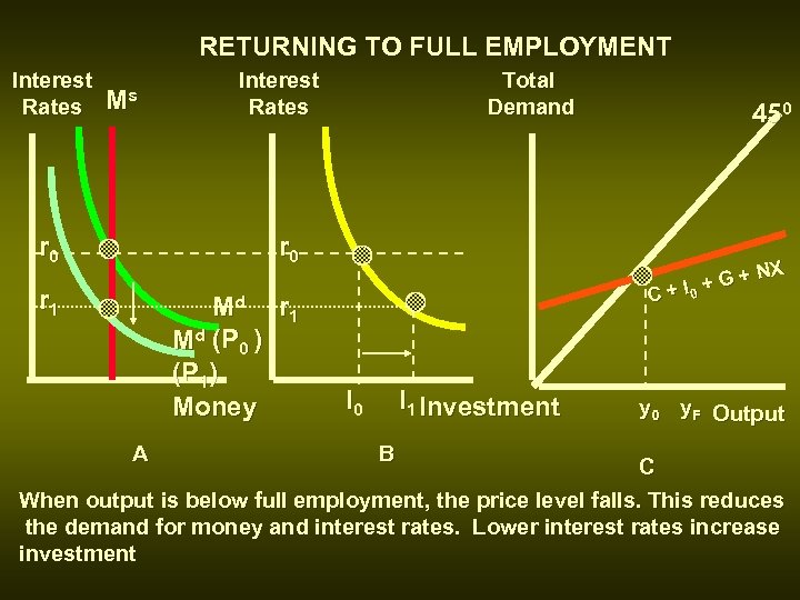RETURNING TO FULL EMPLOYMENT Interest Rates Ms Interest Rates r 0 Md r 1 Md (P 0 ) (P 1) Money 450 r 1 Total Demand A C I 0 I 1 Investment B + I 0 + G + NX y 0 y. F Output C When output is below full employment, the price level falls. This reduces the demand for money and interest rates. Lower interest rates increase investment

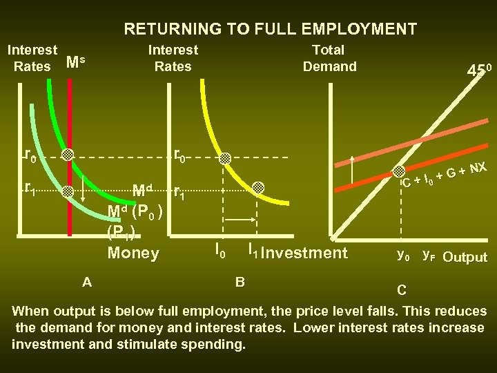RETURNING TO FULL EMPLOYMENT Interest Rates Ms Interest Rates r 0 Md r 1 Md (P 0 ) (P 1) Money 450 r 1 Total Demand A C I 0 I 1 Investment B + I 0 + G + NX y 0 y. F Output C When output is below full employment, the price level falls. This reduces the demand for money and interest rates. Lower interest rates increase investment and stimulate spending.

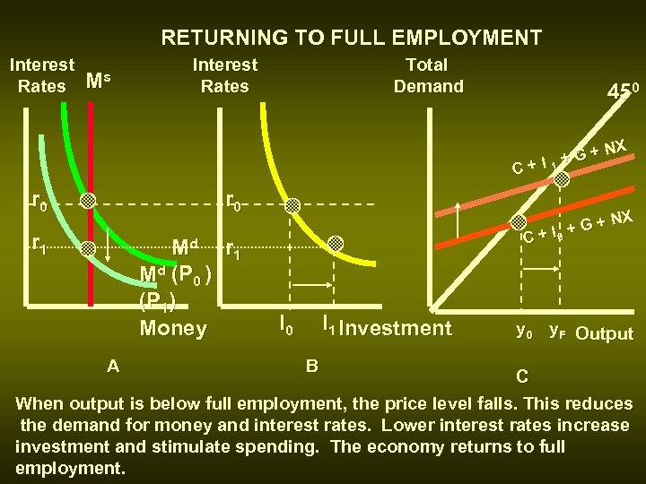RETURNING TO FULL EMPLOYMENT Interest Rates Ms Interest Rates Total Demand 450 G+ +I 1+ C r 0 r 1 Md (P 0 ) (P 1) Money A C I 0 I 1 Investment B NX + I 0 + G + NX y 0 y. F Output C When output is below full employment, the price level falls. This reduces the demand for money and interest rates. Lower interest rates increase investment and stimulate spending. The economy returns to full employment.

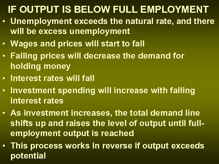IF OUTPUT IS BELOW FULL EMPLOYMENT • Unemployment exceeds the natural rate, and there will be excess unemployment • Wages and prices will start to fall • Falling prices will decrease the demand for holding money • Interest rates will fall • Investment spending will increase with falling interest rates • As investment increases, the total demand line shifts up and raises the level of output until fullemployment output is reached • This process works in reverse if output exceeds potential

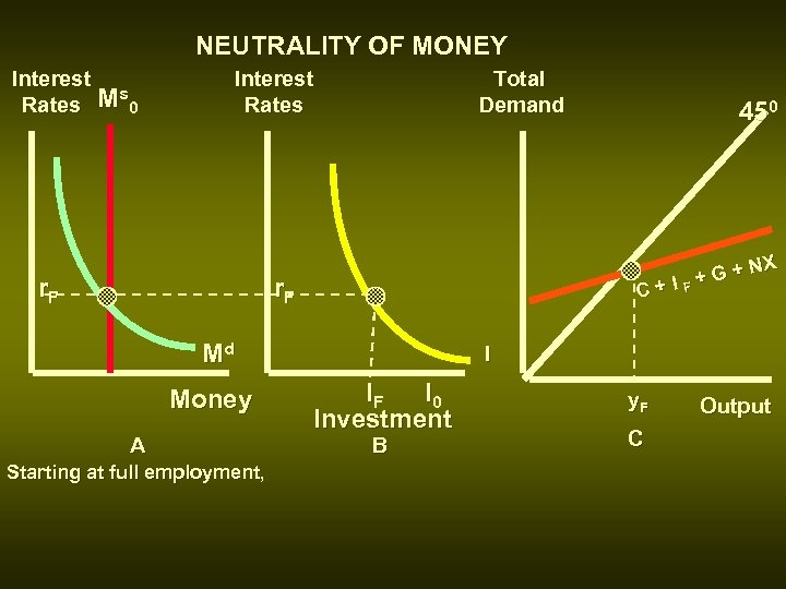NEUTRALITY OF MONEY Interest s Rates M 0 Interest Rates r. F Total Demand + I F+G C+ r. F Md Money A Starting at full employment, 450 NX I IF I 0 Investment B y. F C Output

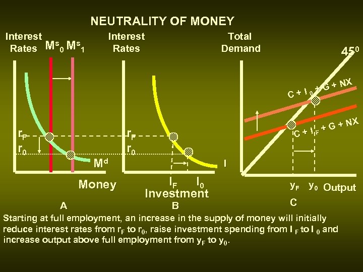NEUTRALITY OF MONEY Interest s s Rates M 0 M 1 Interest Rates Total Demand 450 G+ +I 0+ C r. F r 0 Md Money A NX + I F+G C+ r. F r 0 NX I IF I 0 Investment B y. F y 0 Output C Starting at full employment, an increase in the supply of money will initially reduce interest rates from r. F to r 0, raise investment spending from I F to I 0 and increase output above full employment from y. F to y 0.

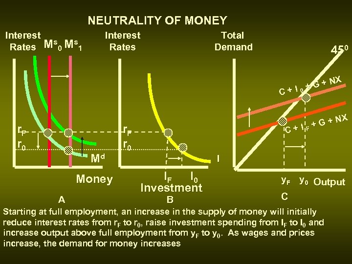NEUTRALITY OF MONEY Interest s s Rates M 0 M 1 Interest Rates Total Demand 450 G+ +I 0+ C r. F r 0 Md Money A NX + I F+G C+ r. F r 0 NX I IF I 0 Investment B y. F y 0 Output C Starting at full employment, an increase in the supply of money will initially reduce interest rates from r. F to r 0, raise investment spending from IF to I 0 and increase output above full employment from y. F to y 0. As wages and prices increase, the demand for money increases

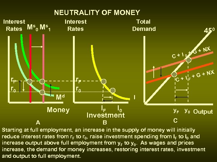NEUTRALITY OF MONEY Interest s s Rates M 0 M 1 Interest Rates Total Demand 450 G+ +I 0+ C r. F r 0 Md Money A NX + I F+G C+ r. F r 0 NX I IF I 0 Investment B y. F y 0 Output C Starting at full employment, an increase in the supply of money will initially reduce interest rates from r. F to r 0, raise investment spending from IF to I 0 and increase output above full employment from y. F to y 0. As wages and prices increase, the demand for money increases, restoring interest rates, investment and output to full employment.

• • LONG-RUN EFFECTS OF AN INCREASE IN THE MONEY SUPPLY If the economy is at full employment and the Bank increases the money supply: In the Short Run Interest rates will decline The level of investment spending will increase The increased demand for output will raise the output above full employment In the Long Run Wages and prices will start to increase The demand for money will increase Interest Rates will increase Investment will start to fall and output will fall

LONG-RUN NEUTRALITY OF MONEY In the long run, increases in the supply of money have no effect on real variables, only on prices.