Convolution 1 D To convolves two vectors u

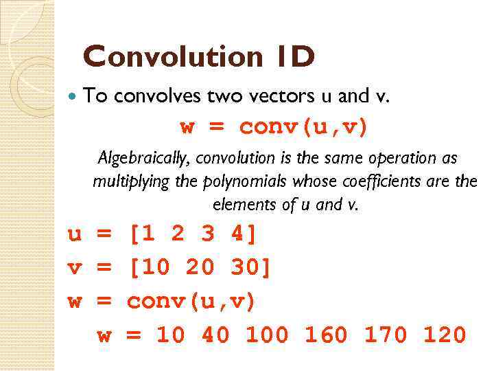Convolution 1 D To convolves two vectors u and v. w = conv(u, v) Algebraically, convolution is the same operation as multiplying the polynomials whose coefficients are the elements of u and v. u = [1 2 3 4] v = [10 20 30] w = conv(u, v) w = 10 40 100 160 170 120

Convolution 1 D u = [1 2 3 4] v = [10 20 30] w = 10 40 100 160 170 120 u 1 2 3 4 30 20 10 10 40 100 160 170 120

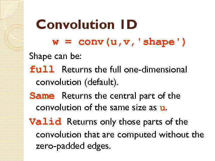Convolution 1 D w = conv(u, v, 'shape') Shape can be: full Returns the full one-dimensional convolution (default). Same Returns the central part of the convolution of the same size as u. Valid Returns only those parts of the convolution that are computed without the zero-padded edges.

Convolution 1 D u = [1 2 3 4] v = [10 20 30] %inv. order Full (default) w = 10 40 100 160 170 120 Same w = 40 100 160 170 Valid w = 100 160

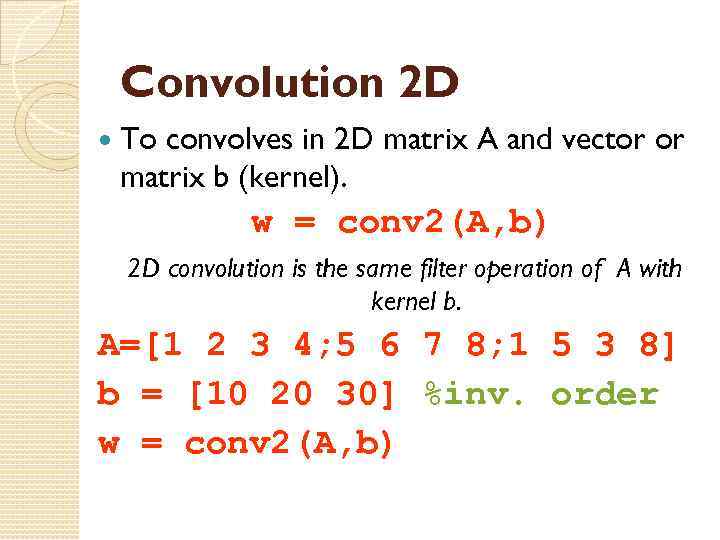Convolution 2 D To convolves in 2 D matrix A and vector or matrix b (kernel). w = conv 2(A, b) 2 D convolution is the same filter operation of A with kernel b. A=[1 2 3 4; 5 6 7 8; 1 5 3 8] b = [10 20 30] %inv. order w = conv 2(A, b)

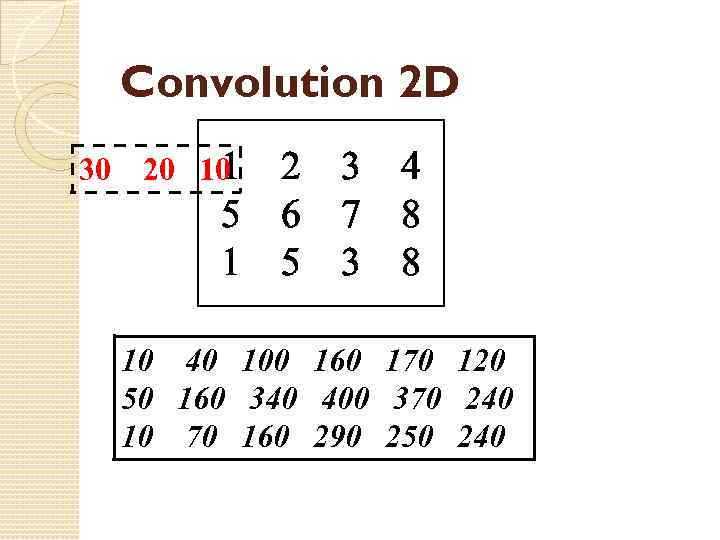Convolution 2 D 30 1 20 10 2 5 6 1 5 3 7 3 4 8 8 10 40 100 160 170 120 50 160 340 400 370 240 10 70 160 290 250 240 100 160 170 120

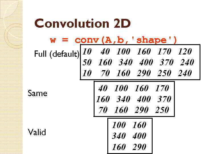Convolution 2 D w = conv(A, b, 'shape') Full (default) 10 40 100 160 170 120 50 160 340 400 370 240 10 70 160 290 250 240 Same Valid 40 100 160 170 160 340 400 370 70 160 290 250 100 160 340 400 160 290

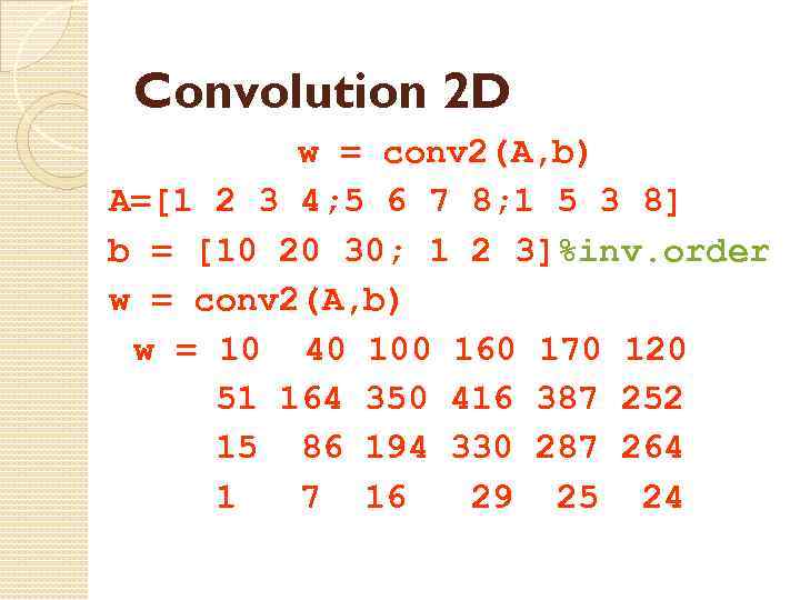Convolution 2 D w = conv 2(A, b) A=[1 2 3 4; 5 6 7 8; 1 5 3 8] b = [10 20 30; 1 2 3]%inv. order w = conv 2(A, b) w = 10 40 100 160 170 120 51 164 350 416 387 252 15 86 194 330 287 264 1 7 16 29 25 24

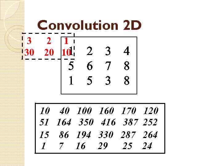Convolution 2 D 3 30 2 1 1 20 10 2 5 6 1 5 3 7 3 4 8 8 10 40 100 160 170 120 51 164 350 416 387 252 15 86 194 330 287 264 1 710 16 29 24 40 10025160 170 120

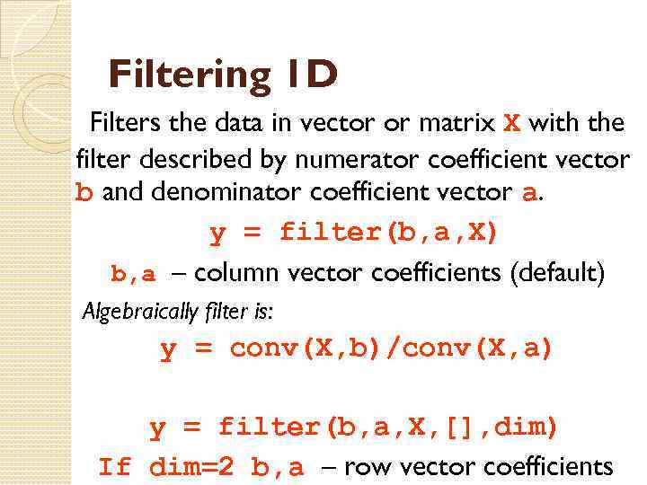Filtering 1 D Filters the data in vector or matrix X with the filter described by numerator coefficient vector b and denominator coefficient vector a. y = filter(b, a, X) b, a – column vector coefficients (default) Algebraically filter is: y = conv(X, b)/conv(X, a) y = filter(b, a, X, [], dim) If dim=2 b, a – row vector coefficients

Filtering 2 D Filters the data in X with the two-dimensional Finite Impulse Response (FIR) filter in the matrix or vector h (kernel). Y = filter 2(h, X) X=[1 2 3 4; 5 6 7 8; 1 5 3 8] h = [10 20 30] %Noinv. order y = filter 2(h, X)

Filtering 2 D Y = filter 2(h, X, 'shape') Shape can be: full Returns the full two-dimensional convolution. Same Returns the central part of the convolution of the same size as X (default). Valid Returns only those parts of the convolution that are computed without the zero-padded edges.

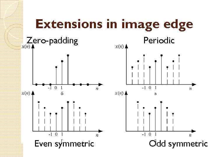Extensions in image edge Zero-padding Even symmetric Periodic Odd symmetric

Discrete Fourier Transform 1 D By default, MATLAB’s fft(X) command outputs X(ej 2 pk/N) for 0 <= 2 pk/N < 2 p Centered Specter: To get the output into the standard range of –p to p, use the fftshift() Y=fft(X); abs. Y=abs(Y); YC = fftshift(abs. Y) r. Fc = real(Y); i. Fc = imag(Y); Fase. Fc= atan(i. Fc. /r. Fc);

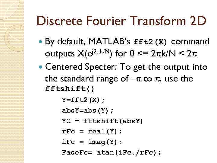Discrete Fourier Transform 2 D By default, MATLAB’s fft 2(X) command outputs X(ej 2 pk/N) for 0 <= 2 pk/N < 2 p Centered Specter: To get the output into the standard range of –p to p, use the fftshift() Y=fft 2(X); abs. Y=abs(Y); YC = fftshift(abs. Y) r. Fc = real(Y); i. Fc = imag(Y); Fase. Fc= atan(i. Fc. /r. Fc);

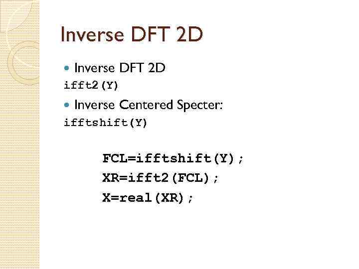Inverse DFT 2 D Inverse DFT ifft 2(Y) 2 D Inverse Centered ifftshift(Y) Specter: FCL=ifftshift(Y); XR=ifft 2(FCL); X=real(XR);