Controlling the future lessons from Quantum Mechanics

Скачать презентацию Controlling the future lessons from Quantum Mechanics

3b31c367e58f7301cd7203db1d72374d.ppt

Количество слайдов: 131

Controlling the future – lessons from Quantum Mechanics “Prediction is a difficult thing – especially of the future” - Nils Bohr

Controlling the future – lessons from Quantum Mechanics “Prediction is a difficult thing – especially of the future” - Nils Bohr “All is foreseen but permission is granted” – The Talmud

Controlling the future – lessons from Quantum Mechanics “Prediction is a difficult thing – especially of the future” - Nils Bohr “All is foreseen but permission is granted” – The Talmud Is the future determined? If yes, can we predict it? If yes, can we control it?

Newtonian Mechanics: Given the position and velocity of a macroscopic body in the present we can use Newton’s second law F=ma where F is the force acting on the body, m is it its mass, and a is the acceleration, to calculate the position and velocity of that body at any time t in the future. present t (future) This can in principle be repeated for each and every particle in the universe, so seemingly, not only is the future determined by the state of the universe in the present but we ought to be able to predict where it is going by solving Newton’s second law equation.

earth sun In practice we can only calculate the trajectories of simple systems (e. g. , a planet orbiting the sun) over sufficiently long times. When more bodies are involved, in most cases the motion becomes “chaotic”. When chaos occurs it is impossible to solve Newton’s equations of motion to sufficient accuracy: the further in the future we inquire, the better do we need to know the present positions and velocities of all bodies involved. The degree of accuracy of our knowledge of the present must increase exponentially, the further in time we desire to predict the future.

pocket An example: Set N billiard balls along a straight line and try to hit the first billiard ball such that the last one is pocketed. This becomes exponentially more difficult with N.

pocket pocket

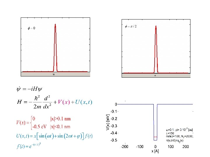
Quantum Mechanics: Quantum Mechanics describes the motion of microscopic bodies (e. g. , an electron, a photon, an atom, a molecule). The equations of motion are those of waves (“wave functions”). These equations do not give rise to chaotic behavior: Given the wave function in the present we can calculate its value at any time in the future to sufficient accuracy even when a large number (hundreds) of microscopic bodies are involved. Does that mean that Quantum Mechanics allows us to predict the future? Not necessarily. The wave function tells us about the whereabouts of the particle only in a statistical way: It tells us what we are likely to observe, i. e. , what is the distribution of outcomes when we repeat the same experiment many times.

Waves and phases angle= 0 o Circular motion Projection on a line 0 o amplitude (=length of projection) phase (=angle)

phase phase

180 o 0 o phase 180 o

0 o phase 180 o

360 o 0 o phase 180 o 360 o

360 o 0 o phase + 180 o - 360 o

+ amplitude phase -

+ wave function phase + probability = wave function 2 probability phase

given the wave function at present (t=0) we can calculate the wave function in the future (t=1 ps)

Interference between waves going through two slits

+ + - a + + + b + -

Screen + a + 0 “destructive” “constructive” b + 0 - + - “destructive”

Screen + a b + + 0 0 - + - Probability

P = (a+b)2 = a 2 + b 2 + 2 ab If a=b then P=4 a 2 If a= - b then - P=0 + + 0 P=0 a P=4 a 2 b + 0 - + -

But this interference pattern is never seen in any individual event! + a b + + 0 0 - + -

+ a b + + 0 0 - + -

Screen + a + 0 Probability b + 0 - + -

How then can we control the outcome of microscopic events. e. g. chemical reactions? H-O + D H O D Cleave the O-D bond H + O-D Cleave the O-H bond Or in greater generality: B A-B + C A Cleave the B-C bond C A + B-C Cleave the A-B bond where A, B, or C can be any atom or any group of atoms.

let a matter wave (particle)

let a matter wave (particle) interact with a light wave

“Entangling” light and matter waves matter wave light wave amplitude for the particle to absorb the light wave and be excited

light wave a

light wave a matter wave

light wave a amplitude for absorbing light wave a

phase shift light wave a amplitude for absorbing light wave a light wave b

phase shift light wave a amplitude for absorbing light wave a light wave b amplitude for absorbing light wave b

phase shift light wave a amplitude for absorbing light wave a interfere light wave b matter wave after absorption of light wave b

The key to control is that the interference patterns of different outcomes be shifted in phase. A-B + C the “screen” of phases A + B-C - is favored

A-B + C A + B-C - is favored

How does it work in real experiments?

Control of the direction of electronic motion: current without voltage!

“slit” a “slit” b

Polar plots: a way of plotting angular distributions Distance from origin proportional to magnitude at a given direction - +

Anti-symmetric - + + 1 - photon absorption Symmetric + + 2 - photon absorption or + - + Symmetric

- + + + - + + +

- - + + + - +

forward backward E. Dupont, P. B. Corkum, H. C. Liu, M. Buchanan, and Z. R. Wasilewski, Phys. Rev. Lett. 74, 3596 (1995)

We have thus been able to transform a probabilistic situation to a situation of certainty. This is exactly what happens when we make a measurement, the wave function with its associated probability “collapses” to a single value which is the “spot” that we see. The main difference is that in a measurement we cannot control where the “spot” appears. + a + 0 “spot” b + - 0 + -

This sheds new light on the very act of measurement: instead of entangling the particle wave with the light wave, the particle to be measured gets entangled with the atoms of the measuring device. It undergoes a similar multi-path interference, whose nature changes constantly and rapidly with time. The particle gets absorbed by a detector atom when its wave function assumes the value of 1 at the position of a given detector atom.

Milestones in the development of “coherent control” blue – theory red - experiments • 1986: Original suggestion to use quantum interference for control. Introduction of the concept “coherent control”. B + A-C 2 A + B-C E E 2 1 E 1 4 3 Eg

1988: (with Hepburn) Introduction of 1 photon vs. 3 photon interference as a means of control B+AC A+BC ABC 1989: (with Kurizki) Introduction of 1 photon vs. 2 photon as a means of symmetry breaking and differential control: prediction of creation of DC photo current in semi conductors with no bias voltage. conduction band backward e- forward

1990: First experimental verification of the 1 vs. 2 coherent control scenario. Control over photo-current directionality in semiconductors (Zeldovitch) 1990/1991: First experimental verifications of the 1 vs. 3 coherent control scenario: The control of photoionization yields in atoms (Elliott, Bucksbaum) and molecules (Gordon, Bersohn) 1991: Coherent control of molecular chirality introduced

1994/1995: Interference Control with Incoherent light introduced B+AC A+BC - 2 1 1995: Experimental demonstration of coherent control of photo-current generation in quantum wells by the 1 vs. 2 photon scenario (Corkum) 2

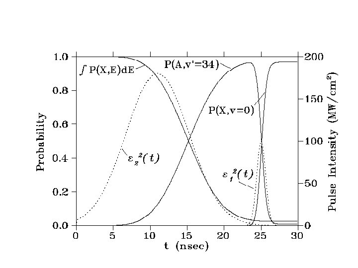
1995: Experimental demonstration of control of electronic hopping in a dissociating molecule, in 1 vs. 2 photon H+ + D HD+ H + D+ (Di. Mauro) 1995: (Gordon) First experimental demonstration of control over a branching process: control over the ionization vs. dissociation in 1 vs. 3 photon HI+ HI H+I 1996: First experimental demonstration of control over electronic branching ratios: interference control with incoherent light in Na + Na(3 p) Na 2 Na + Na(3 d) (Shnitman+Yogev+, Shapiro) 1997: (with Vardi) Photoassociation of ultracold atoms to form ultracold molecules via Coherent Raman Process suggested

1997: First experiments on automated feedback control via pulse shapings (Wilson, Silberberg, Gerber) 1998: Experimental demonstration of coherent control via phase modulation of two photon absorption of atoms (Silberberg) 1998: (Gerber) First experimental demonstration of adaptive feedback control of a branching photochemical reaction: Control over the photodissociation of Fe(CO)5 and Cp + 2 CO +Fe. Cl Cp. Fe(CO)2 Cl Cp. Fe. COCl + CO 2000: Coherent Control of refractive indices introduced 2000: (with Frishman) Enantiomeric purification of chiral racemic mixtures by coherent control techniques

• 2000: Theory of nanoscale deposition on surfaces • 2000: (with Frishman) Coherent Suppression of spontaneous emission using overlapping resonances 2001: Adaptive feedback control of the photodissociation of C 6 H 5 CO + CH 3 C 6 H 5 CH 3 CO C 6 H 5 + CH 3 CO in the high field regime (Levis) |2’› |1’› |0› 2002: (with Kral): An exact analytical solution of the non-degenerate quantum control problem |3› |2› |1› 2002: Adaptive feedback control of internal conversion channel in a light harvesting antenna complex of photosynthetic purple bacterium (Motzkus) 2003: (with Kral and Thanopoulos): An analytic solution for the degenerate quantum control problem 2003: (with Zhang and Keil) Experimental demonstration of phase locking between two 2 -photon processes in 2 -photon vs. 2 -photon coherent control 2003 -2004: Experimental control of high harmonic generation (Murnane, Gerber)

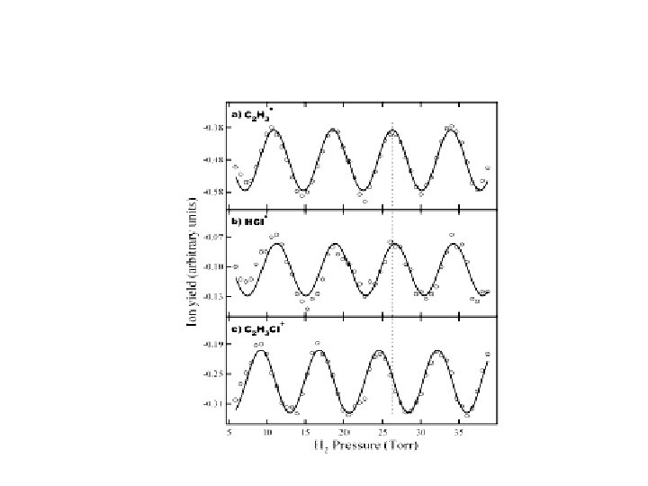
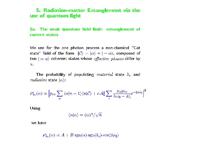
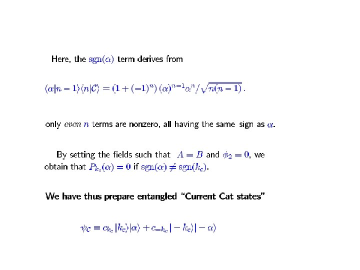
2004: Coherent Control techniques used in the “streak camera” phase measurement attosecond pulses (Krausz, Corkum) e +E -E • 2005: Control of radiationless transitions by interference between overlapping resonances 2005: (with Thanopoulos) Automatic repair of mutations caused by dihydrogenic tunneling between two nucleotides using coherent control 2005: (with Kral) Coherent control with non-classical light 2005: Experimental demonstration of coherent photoassociation of Rb + Rb BEC to form Rb 2 molecular BEC using the Vardi+Shapiro scheme (Grimm) 2005: Experimental demonstration of bond breaking selectivity in the CH 2=CH. + Cl CH 2=CHCl CH= CH + HCl (Gordon) 2005: (with Segal) Suggestion of quantum computation using electron trapped in an quadrupoles of carbon nanotubes e

Barge Vishal J. , Zhan Hu, and Robert J. Gordon, J. Chem. Phys. - submitted J

Control of chirality: The importance of the “envelope phase” The D 2 S 2 chiral isomers

The purification of a mixture of molecules with opposite handedness by optical means (Phys. Rev. Lett. 84, 1669 (2000)

1 2 A. Vardi, D. Abrashkevitch, E. Frishman, and M. Shapiro, J. Chem. Phys. 107, 6166 (1997)

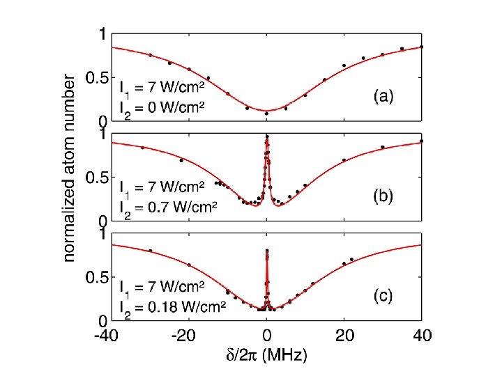
Coherent Raman photoassociation of Rb+Rb Rb 2 K. Winkler, G. Thalhammer, M. Theis, H. Ritsch, R. Grim, and J. Hecker Denschlag, Cond-mat/0505732 v 1 30 May 2005

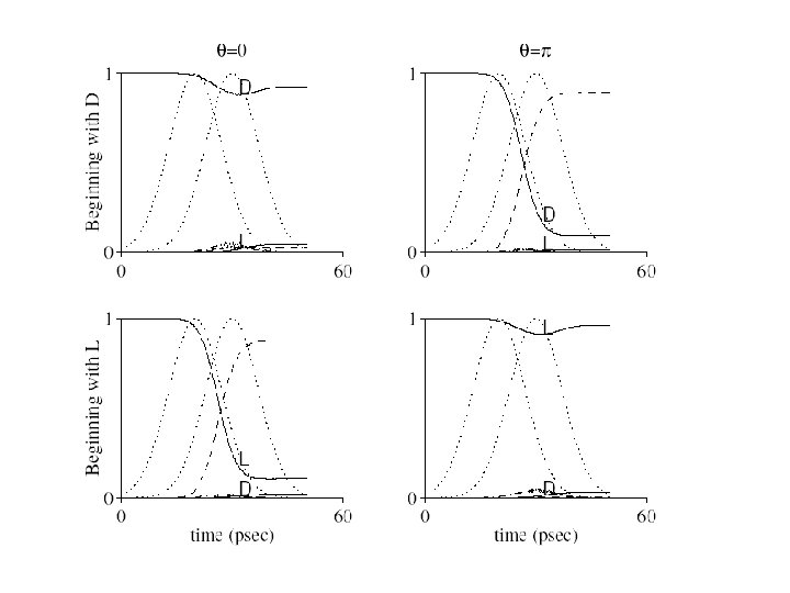
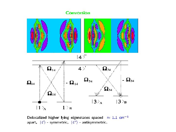
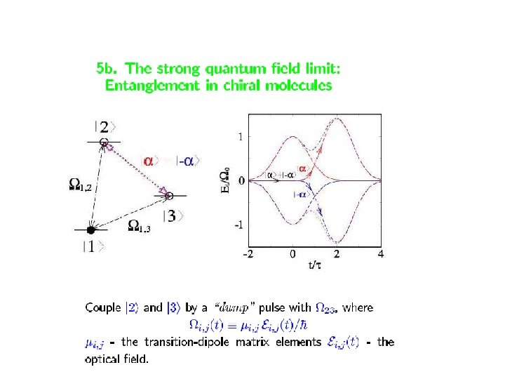
“Loop” adiabatic passage in chiral molecules The D 2 S 2 chiral isomers

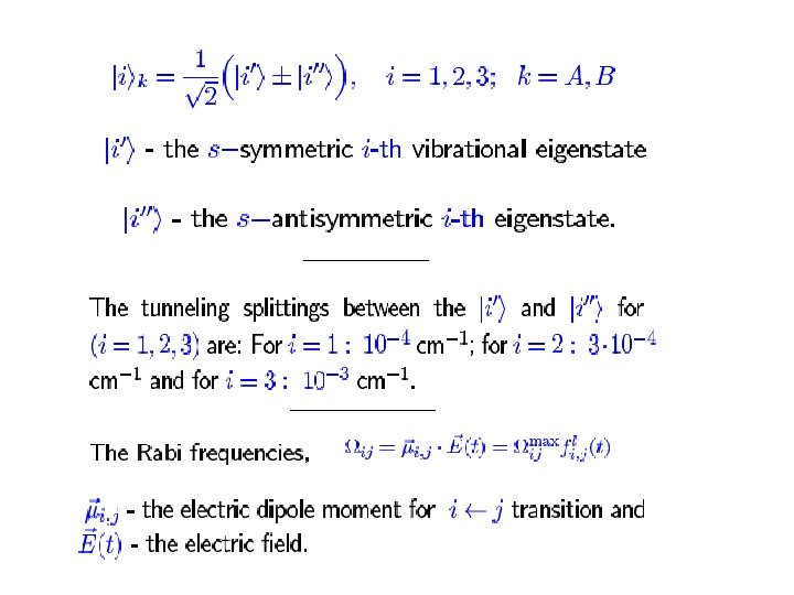
Symmetry breaking in loop systems In the loop system the eigenvalues depend on the phases

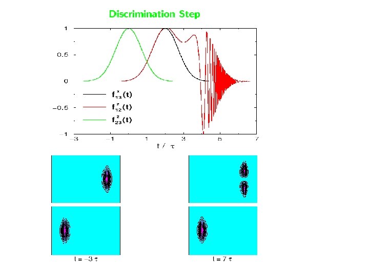
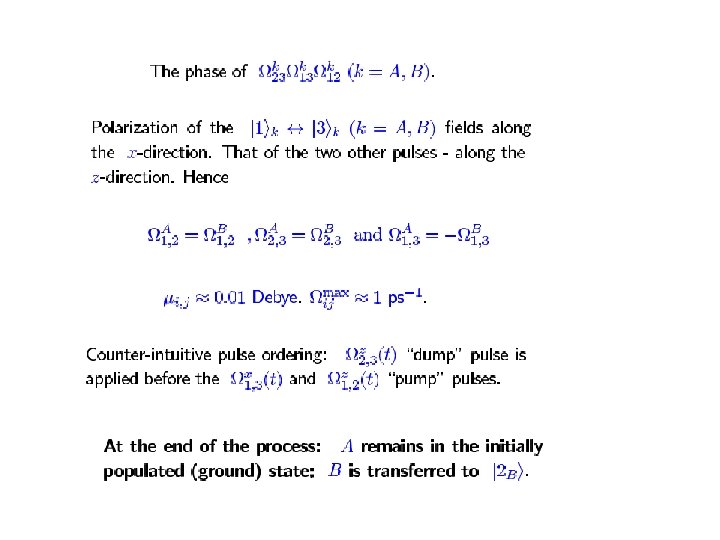
The dependence of the population transfer on the phase

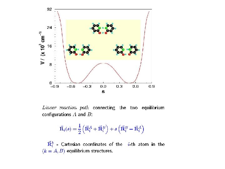
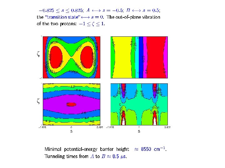
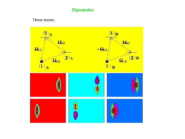
Detection and automatic repair of mutations by coherent light Dihydrogenic tunneling in a dinucleotide pair I. Thanopoulos and M. Shapiro, J. A. C. S. – in press

Tubular image states (TIS) §Suspended linear molecular conductors or dielectrics support highly-extended electronic states. §The electron is attracted to the material surface by its image charge and repelled by a centrifugal force due to its rotational motion. §The combination of these two effects yields effective potential curves having long range (10 -50 nm) potential wells that support bound states that are separated from the surface, and can have long lifetimes at low temperatures. B. E. Granger, P. Král, H. R. Sadeghpour and M. Shapiro, PRL 89, 135506 (2002).

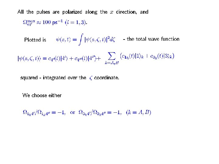
The origin of attraction of TIS §The stability of TIS is due to interplay between the attractive image potential and repulsive centrifugal potentials §Close to the surface the centrifugal potential and Coulomb attraction give rise to 1 -2 e. V barriers §The total wave functions and eigenenergies:

Potential Energy for Finite Segmented Systems Attractive part of the potential N=2 -8 Total potential N=2 at z=0 N=8 Detached local minimum

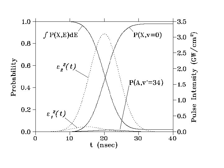
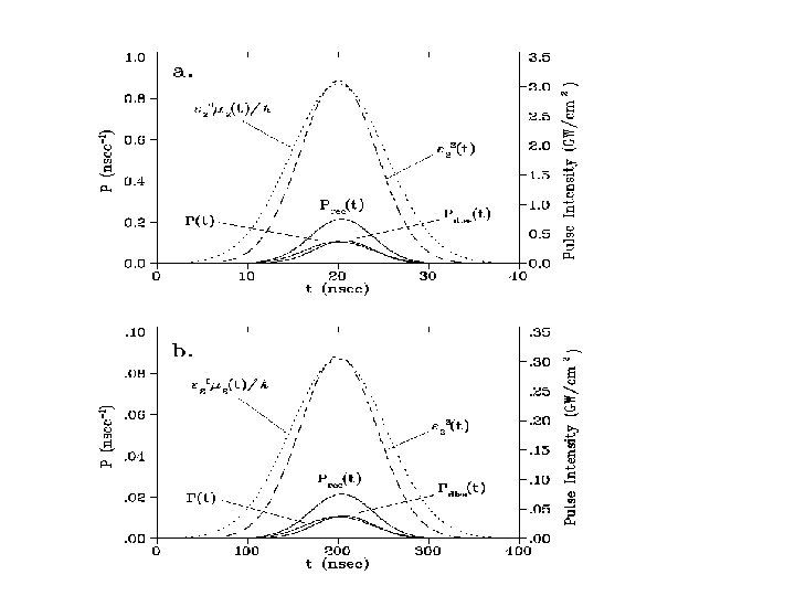
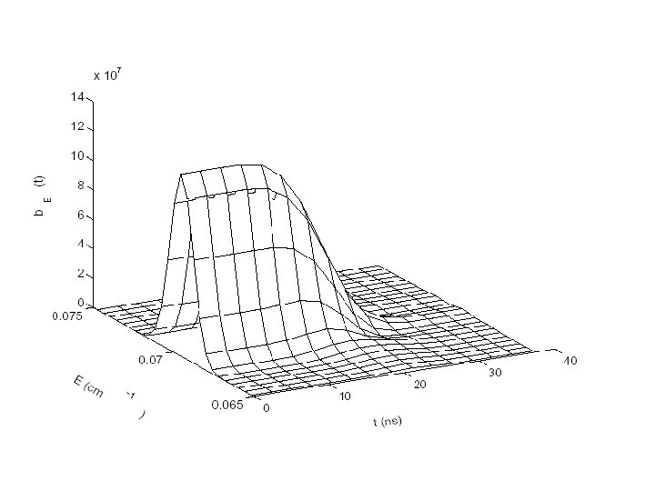
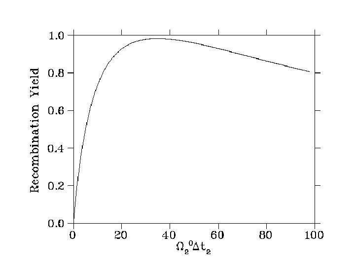
Optically induced electron transfer over barriers Hopping of electrons over potential barriers with no net absorption of photons by implementing the Laser catalysis scenario. Switch! e A. Vardi, M. Shapiro, Phys. Rev. A 58, 1352 (1998).

Image states bands over suspended arrays of nanowires • We have studied TIS above nanotube arrays • The states can remain largely detached and form bands. B. E. Granger, D. Segal, H. R. Sadeghpour, P. Král and M. Shapiro, PRL, 94, 016402 (2005) Z. P. Huang et. al. App. Phys. Lett. 82, 460 (2003)

Coherent Control as a Disentanglement Transformation

Acknowledgments Theory Ioannis Thanopulos (Univ. of British Columbia) Einat Frishman (Univ. of British Columbia) Petr Kral (Univ. Illinois at Chicago) Dvira Segal (Weizmann ) Paul Brumer (University of Toronto) John Hepburn (University of British Columbia) Ilya Averbukh (Weizmann) Experiment Qun Zhang (Weizmann, now at Univ. of British Columbia) Alexander Shnitman (Weizmann) , Mark Keil (BGU)