Consumer choice based on the textbooks written by

Consumer choice (based on the textbooks written by Colander, Hyman and Mc. Connell & Brue) 1

Central question of the topic… n n Say you’re a junk food devotee. You live on two goods: chocolate bars and cans of cola. That’s all you purchase. In making your consumption choices, you’re trying to get as much pleasure as possible. The question is: HOW MANY CHOCO BARS AND COLA CANS DO YOU CHOOSE IN A GIVEN TIME INTERVAL? 2

…and answer to the question n The answer is: IT DEPENDS ON TWO THINGS: q q n BUDGET CONTRAINTS (INCOME AND PRICES), PREFERENCES (TASTES). Note that all of them are key demand determinants. 3

Practical dimension n Individual benefits: the understanding of the way we make our consumption choices can help us spend our money in more fruitful ways Institutional benefits: the understanding of the way we make our consumption choices can help firms make more appropriate sales decisions Other benefits: better understanding of observed behavior (new consumption patterns) 4

Initial assumptions (quite reasonable, aren’t they? ) n n In making consumption choices, you’re going to maximize your utility You prefer to have more than less You’re able to value affordable baskets of goods from the point of view of their utilities Your choices are rational 5

First step in the analysis: the contraints part n n Income (per week): I = $50 Price of choco bar: PCHOCO = $5 Price of cola can: PCOLA = $10 Before you make the consumption decision, you must figure out affordable budget options 6

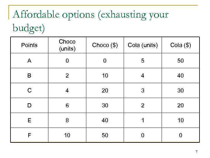
Affordable options (exhausting your budget) Points Choco (units) Choco ($) Cola (units) Cola ($) A 0 0 5 50 B 2 10 4 40 C 4 20 3 30 D 6 30 2 20 E 8 40 1 10 F 10 50 0 0 7

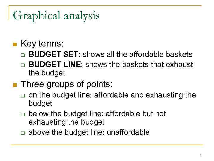
Graphical analysis n Key terms: q q n BUDGET SET: shows all the affordable baskets BUDGET LINE: shows the baskets that exhaust the budget Three groups of points: q q q on the budget line: affordable and exhausting the budget below the budget line: affordable but not exhausting the budget above the budget line: unaffordable 8

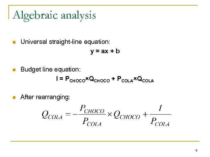
Algebraic analysis n Universal straight-line equation: y = ax + b n Budget line equation: I = PCHOCO×QCHOCO + PCOLA×QCOLA n After rearranging: 9

Combined graphic and algebraic analysis n n Suppose your weekly income increases from $50 to $60. Suppose price of choco bar doubles. Suppose price of cola can drops to $5. In each of these three cases – what is the effect on budget line equation and location? 10

Market trade-off and price ratio n n The budget line shows the MARKET TRADE-OFF between two goods (choco bars ans cola cans in our case). The market trade-off is reflected in relation of prices (PRICE RATIO or RELATIVE PRICE). In our case it is -1/2 meaning that, at assumed market prices of choco bars and cola cans, each time you want to buy one more cola can you have to divert $10 from choco purchases, reducing the number of $5 choco bars you can purachse by 2. 11

Market trade-off and price ratio in a nutshell n n To get one additional cola can in the market you have to resign two choco bars. That’s the market trade-off you have to obey. Seen from this perspective, price ratio should be considered an OPPORTUNITY COST of having (cosuming) a good. 12

Budget constraint is just part of the story n Now that we know all baskets within your reach, the following question arises: WHICH ONE DO YOU ACTUALLY CHOOSE? A, B, C, D, E or F? n To answer the question we need another factor: your preferences. 13

Second step in the analysis: the pleasure part n n n Key term: INDIFFERENCE CURVE („Just-as-happy curve”) Indifference curve: a curve showing all combinations of two goods (choco bars and cola cans in our case) that generate the same level of utility. Let’s explore indifference curves in three steps that are devoted to: q q q how are they plotted, what are their properties, how do they relate to preferences. 14

Plotting the indifference curves n n Imagine that you choose randomly a point that illustrates a basket of two goods. All other baskets can be categorized into: q q q superior (preferred) combinations, inferior (not preferred) combinations, equivalent. 15

Properties of indifference curves n n They’re downward sloped: as budget line, they show trade-off between two goods, trade -off that must keep your utility constant They’re bowed inward (bowed toward the origin): their shape is consistent with the law of diminishing marginal rate of substitution 16

Marginal rate of substitution (MRS) n Marginal rate of substitution: the quantity of one good (COLA) a consumer would give up to obtain one more unit of another good (CHOCO) while being made neither better off nor worse off by the trade (in other words – assuming that the consumer’s utility doesn’t change). 17

Personal trade-off n n MRS should be considered a personal trade-off between two goods (cola and choco in our case) or the rate at which the consumer is willing to substitute one good for another. Personal trade-off is the answer we would get to the following question: „Say you didn’t know the price of either good and we took away a given amount of one of them. How many units of the other one would we have to give you so that you would be just as happy as before? ” 18

The law of diminishing MRS (quite reasonable, isn’t it? ) n n The law of diminishing marginal rate of substitution: MRS of one good (COLA) for another good (CHOCO) tends to decline as more of one good is substituted for another along any consumer’s indifference curve. People usually don’t like extremes. They prefer balanced consumption. That’s the rationale behind the law. 19

Graphic and algebraic analysis n n In fact, MRS reflects slope of indifference curve at any given point located on the curve As we move along an indifference curve downward (from left to right), MRS declines (the law of diminishing MRS) and the curve becomes more and more flat 20

Properties of indifference curves (cont. ) n n Each indifference curve represents a given level of utility that is constant along the curve. For each consumer, there is infinite number of indifference curves, each with a different level of utility. All of them consitute an INDIFFERENCE MAP. The farther indifference curve is located from the origin, the higher level of utility is represents. Indifference curves can’t cross one another on the indifference map. 21

Utility maximization and indifference map n n Remember your ultimate goal: TO MAXIMIZE UTILITY. By the spoken of indifference curve it means that you want to get to as high indifference curve as possible, given your budget constraint. 22

Indifference curves as a mirror of consumer’s preferences n n Imagine two students having extremely different preferences in our hypothetical twogoods-world. Let’s say that Natasha prefers choco to cola while Boris prefers cola to choco. How would their indifference maps look like? 23

Best affordable choice or consumer equilibrium n n Graphic interpretation: the point on your budget line and on your highest attainable indifference curve; the point at which highest attainable indifference curve touches (is tangent to) your budget line Algebraic interpretation: the point at which slope of your budget line and slope of an indifference curve are the same 24

Best affordable choice or consumer equilibrium (cont. ) n n Economic interpretation: basket of goods for which your personal trade-off (MRS) equals the market trade-off (price ratio). Could you do better? q q When MRS = price ratio NO! When MRS ≠ price ration YES! 25

Historical perspective n n n The way we study consumer choices represents new (modern) school of theoretical research on the subject. Old school was based on the notion of utility measurement. Economists even invented special measurement unit: UTIL. Contemporaneous economists consider the concept questionable and the usage of such „utilometer” is troublesome for them. 26

Behid the scenes goal of our analysis: best affordable choice and demand curve n n We can use indifference analysis to show the effects of changes in price of one of the two goods on the quantity demanded of the good. This then enables us to derive an individual’s demand curve for that good. In that way our analysis can explain the law of demand. 27