510070c89dbdffbc95979e658c16107c.ppt
- Количество слайдов: 27
![Consumer Behavior Lecture 8 [Chapter 7] Mc. Graw-Hill/Irwin Copyright © 2009 by The Mc. Consumer Behavior Lecture 8 [Chapter 7] Mc. Graw-Hill/Irwin Copyright © 2009 by The Mc.](https://present5.com/presentation/510070c89dbdffbc95979e658c16107c/image-1.jpg)
Consumer Behavior Lecture 8 [Chapter 7] Mc. Graw-Hill/Irwin Copyright © 2009 by The Mc. Graw-Hill Companies, Inc. All rights reserved.
Chapter Objectives 1. 2. 3. 4. 5. About total utility, marginal utility, and the law of diminishing marginal utility. How rational consumers compare marginal utility-to -price ratios for products in purchasing combinations of products that maximize their utility. How a demand curve can be derived by observing the outcomes of price changes in the utilitymaximization model. How the utility-maximization model helps highlight the income and substitution effects of a price change. About budget lines, indifference curves, utility maximization, and demand derivation in the indifference curve model of consumer behavior. (Appendix) 7 -2

Utility is want-satisfying power a good possesses or the satisfaction or pleasure one receives from consuming a good or service. Diminishing marginal utility (again) Three characteristics › Differs from usefulness › Subjective › Difficult to quantify 7 -3
Law of Diminishing Marginal UItility Explains downward sloping demand Predicts that added satisfaction declines as a consumer acquires additional units of a given product. 7 -4
Total Utility and Marginal Utility Total utility is the total amount of satisfaction or pleasure a person derives from consuming some specific quantity of a good or service. Marginal utility is the extra satisfaction a consumer realizes from an additional unit of that product. Alternatively, marginal utility is the change in total utility that results from the consumption of 1 more unit of a product.
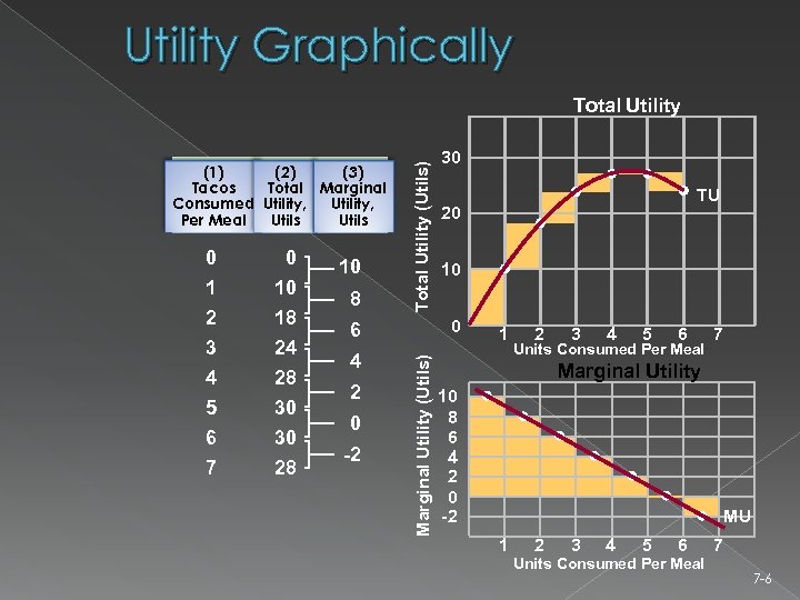
Utility Graphically (1) (2) (3) Tacos Total Marginal Consumed Utility, Per Meal Utils 1 2 3 4 5 6 7 0 ] 18 ] 24 ] 28 ] 30 ] 28 10 8 4 2 0 -2 30 TU 20 10 0 6 Marginal Utility (Utils) 0 Total Utility (Utils) Total Utility 1 2 3 4 5 6 Units Consumed Per Meal 7 Marginal Utility 10 8 6 4 2 0 -2 MU 1 2 3 4 5 6 Units Consumed Per Meal 7 7 -6
Marginal Utility & Demand The law of diminishing marginal utility explains why the demand curve for a given product slopes downward. In the event successive units of a good are consumed with each unit yielding smaller amounts of marginal utility, then the only way a consumer will buy additional amounts of the good is if the price falls.
Theory of Consumer Behavior Key dimensions (assumptions) of the consumer › Consumers engage in Rational behavior › Each consumer has clear cut Preferences › Every consumer faces a Budget constraint › Changes in Prices will alter consumer choices. 7 -8
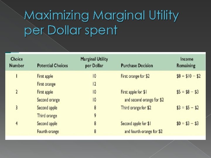
Utility Maximizing Rule Allocate income so that the last dollar spent on each good yields same amount of extra (marginal) utility. When a consumer has ‘balanced his or her margins’ using this rule, he or she has received consumer equilibrium. 7 -9
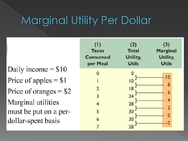
Marginal Utility Per Dollar
Maximizing Marginal Utility per Dollar spent
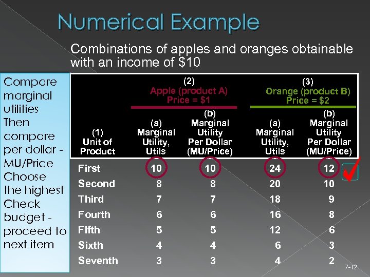
Numerical Example Combinations of apples and oranges obtainable with an income of $10 Compare marginal utilities Then compare per dollar MU/Price Choose the highest Check budget proceed to next item (1) Unit of Product (2) Apple (product A) Price = $1 (b) Marginal (a) Utility Marginal Per Dollar Utility, (MU/Price) Utils (3) Orange (product B) Price = $2 (b) Marginal (a) Utility Marginal Per Dollar Utility, (MU/Price) Utils First Second Third Fourth 10 8 7 6 24 20 18 16 12 10 9 8 Fifth Sixth Seventh 5 4 3 12 6 4 6 3 2 7 -12
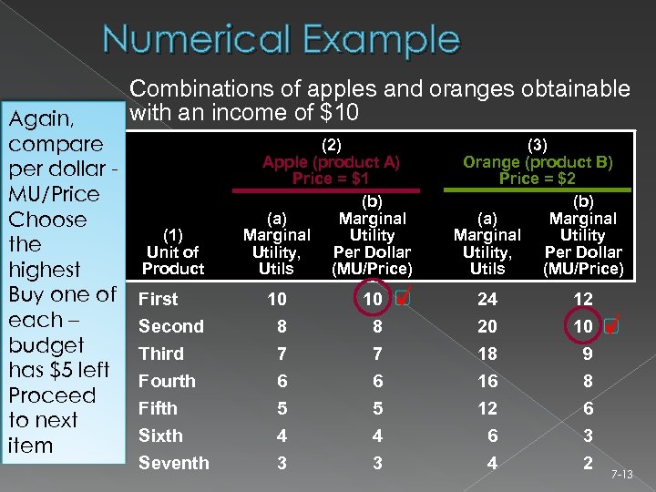
Numerical Example Again, compare per dollar MU/Price Choose the highest Buy one of each – budget has $5 left Proceed to next item Combinations of apples and oranges obtainable with an income of $10 (1) Unit of Product (2) Apple (product A) Price = $1 (b) Marginal (a) Utility Marginal Per Dollar Utility, (MU/Price) Utils (3) Orange (product B) Price = $2 (b) Marginal (a) Utility Marginal Per Dollar Utility, (MU/Price) Utils First Second Third Fourth 10 8 7 6 24 20 18 16 12 10 9 8 Fifth Sixth Seventh 5 4 3 12 6 4 6 3 2 7 -13
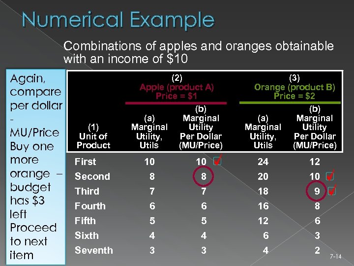
Numerical Example Combinations of apples and oranges obtainable with an income of $10 Again, compare per dollar MU/Price Buy one more orange – budget has $3 left Proceed to next item (1) Unit of Product (2) Apple (product A) Price = $1 (b) Marginal (a) Utility Marginal Per Dollar Utility, (MU/Price) Utils (3) Orange (product B) Price = $2 (b) Marginal (a) Utility Marginal Per Dollar Utility, (MU/Price) Utils First Second Third Fourth 10 8 7 6 24 20 18 16 12 10 9 8 Fifth Sixth Seventh 5 4 3 12 6 4 6 3 2 7 -14
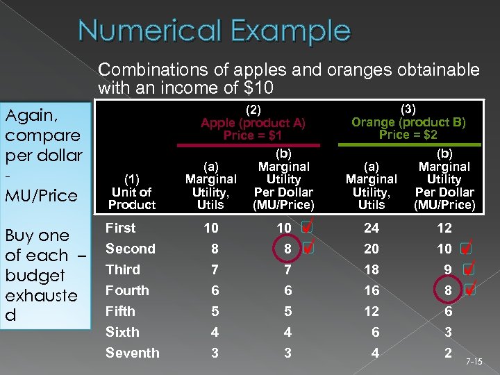
Numerical Example Combinations of apples and oranges obtainable with an income of $10 Again, compare per dollar MU/Price Buy one of each – budget exhauste d (1) Unit of Product (2) Apple (product A) Price = $1 (b) Marginal (a) Utility Marginal Per Dollar Utility, (MU/Price) Utils (3) Orange (product B) Price = $2 (a) Marginal Utility, Utils (b) Marginal Utility Per Dollar (MU/Price) First Second Third Fourth 10 8 7 6 24 20 18 16 12 10 9 8 Fifth Sixth Seventh 5 4 3 12 6 4 6 3 2 7 -15
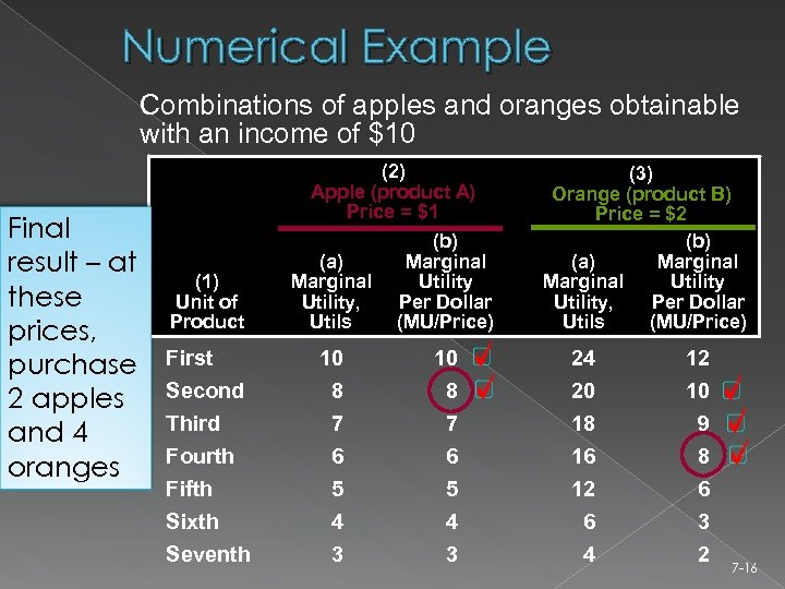
Numerical Example Combinations of apples and oranges obtainable with an income of $10 Final result – at these prices, purchase 2 apples and 4 oranges (2) Apple (product A) Price = $1 (3) Orange (product B) Price = $2 (b) Marginal (a) Utility Marginal Per Dollar Utility, (MU/Price) Utils (1) Unit of Product (a) Marginal Utility, Utils (b) Marginal Utility Per Dollar (MU/Price) First Second Third Fourth 10 8 7 6 24 20 18 16 12 10 9 8 Fifth Sixth Seventh 5 4 3 12 6 4 6 3 2 7 -16
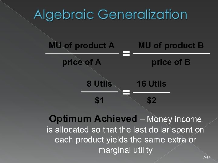
Algebraic Generalization MU of product A price of A 8 Utils $1 = = MU of product B price of B 16 Utils $2 Optimum Achieved – Money income is allocated so that the last dollar spent on each product yields the same extra or marginal utility 7 -17
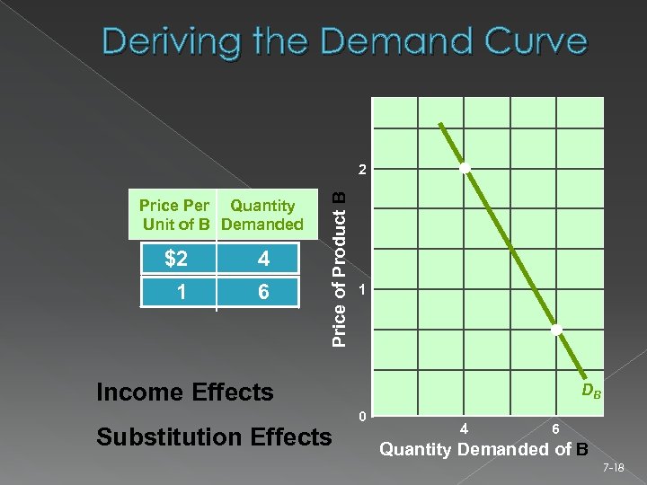
Deriving the Demand Curve Price Per Quantity Unit of B Demanded $2 4 1 6 Price of Product B 2 1 Income Effects Substitution Effects DB 0 4 6 Quantity Demanded of B 7 -18
Income & Substitution Effects Income effect: the impact that a change in a product’s price has on a consumer’s real income and on the quantity demanded of that good. Substitution effect: the impact that a change in a product’s price has on its relative expensiveness and on the quantity demanded

Applications and Extensions New products increase utility › i. Pods The diamond-water paradox The value of time Medical care purchases Cash and noncash gifts 7 -20
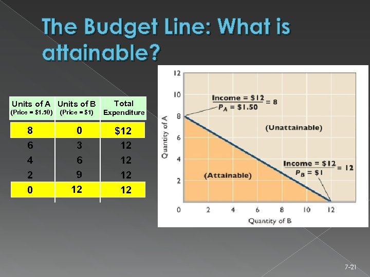
The Budget Line: What is attainable? Units of A Units of B Total (Price = $1. 50) (Price = $1) Expenditure 8 6 4 2 0 0 3 6 9 12 $12 12 12 7 -21
Characteristics of the Budget Line Changes in Money income › An increase in money income shifts the budget line to the right; a decrease in money income shifts it to the left Changes in Prices › a change in product prices also shifts the budget line.
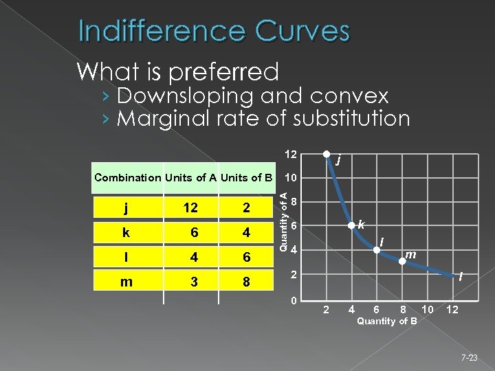
Indifference Curves What is preferred › Downsloping and convex › Marginal rate of substitution 12 j 12 2 k 6 4 l 4 6 m 3 8 10 Quantity of A Combination Units of A Units of B j 8 k 6 l 4 m 2 0 I 2 4 6 8 Quantity of B 10 12 7 -23
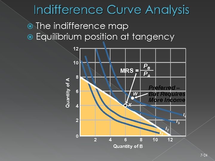
Indifference Curve Analysis The indifference map Equilibrium position at tangency 12 10 MRS = Quantity of A 8 6 W X 4 PB PA Preferred – But Requires More Income I 4 2 0 I 3 I 1 2 4 6 8 Quantity of B 10 I 2 12 7 -24
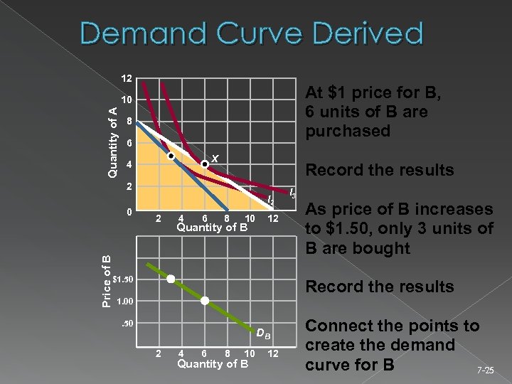
Demand Curve Derived 12 At $1 price for B, 6 units of B are purchased Quantity of A 10 8 6 X 4 Record the results 2 I 2 Price of B 0 2 4 6 8 10 Quantity of B 12 $1. 50 I 3 As price of B increases to $1. 50, only 3 units of B are bought Record the results 1. 00. 50 DB 2 4 6 8 10 Quantity of B 12 Connect the points to create the demand curve for B 7 -25
Key Terms Law of diminishing marginal utility Utility Total utility Marginal utility Rational behavior Budget constraint Utility maximizing rule Income effect Substitution effect 7 -26
Appendix Key Terms Budget Line Indifference curve Marginal rate of substitution (MRS) Indifference map Equilibrium position 7 -27
510070c89dbdffbc95979e658c16107c.ppt