Connectivity Properties for Topology design in Sparse Wireless

Connectivity Properties for Topology design in Sparse Wireless Multi-hop Networks Ph. D. Defense Srinath Perur Advisor: Sridhar Iyer IIT Bombay

Introduction 2

Multi-hop Wireless Networks (MWN) • Multi-hop Wireless Network • • Decentralised Infrastructure-less Cooperative multi-hop routing Examples: • Mobile ad hoc networks • Sensor networks • Mesh networks 3

Topology Design • Combination of network parameters for desired network graph • Ex: Transmission range, area of operation, number of nodes Topology design can be: • Deterministic • Ex: Mesh networks • Probabilistic • Ex: Sensor networks, MANETs 4

Connectivity Properties • Value associated with a network indicating extent to which nodes are connected • Connectivity: probability of nodes forming a single connected component • Size of largest connected component • Connectivity properties are often metrics for topology design • Ex: Transmission range required for a connected network 5

Sparse MWNs • A sparse MWN is one that is not connected with high probability • We assume < 0. 95 • Examples: • Vehicular MWN at low traffic density • Sensor network after some nodes have died • Incrementally deployed MANET • 25/60 sets of network parameters used in Mobi. Hoc papers were sparse 6

Sparse MWNs • Sparse networks can also occur by design • Trade-off connectivity for other network parameters in constrained scenarios • Ex: Delay tolerant networks • Networks tolerating 90% nodes in one connected component required significantly reduced transmission range [SB 03] 7

Questions of Interest • Are currently used connectivity properties appropriate for topology design in sparse MWNs? • How can they be used? • What other connectivity properties can be used? • What trade-offs between network parameters can be made in sparse deployments? • What tools, such as models or simulators, would we require in order to accomplish these tradeoffs while designing networks? 8

Organisation • Connectivity • Empirical characterisation for sparse region in finite domain • Reachability • Definition and properties • Applications • Characterisation • Simran - a topological simulator for MWNs • Spanner - a design tool for sparse MWNs • Edge effects in MWNs • Quantifying the edge effect • Applying it to use results for square area networks in rectangular networks 9

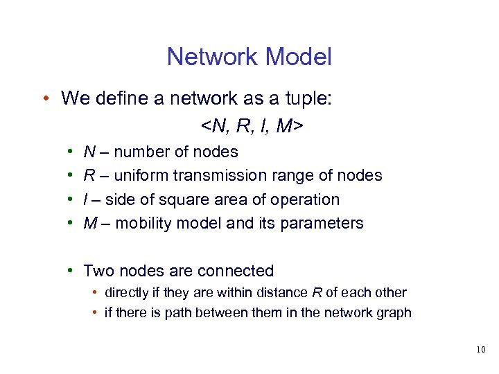Network Model • We define a network as a tuple: • • N – number of nodes R – uniform transmission range of nodes l – side of square area of operation M – mobility model and its parameters • Two nodes are connected • directly if they are within distance R of each other • if there is path between them in the network graph 10

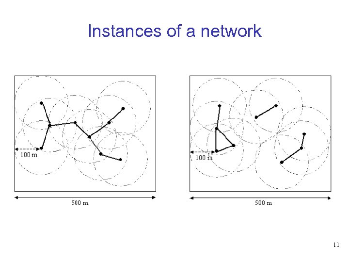Instances of a network 11

Connectivity for Sparse Networks 12

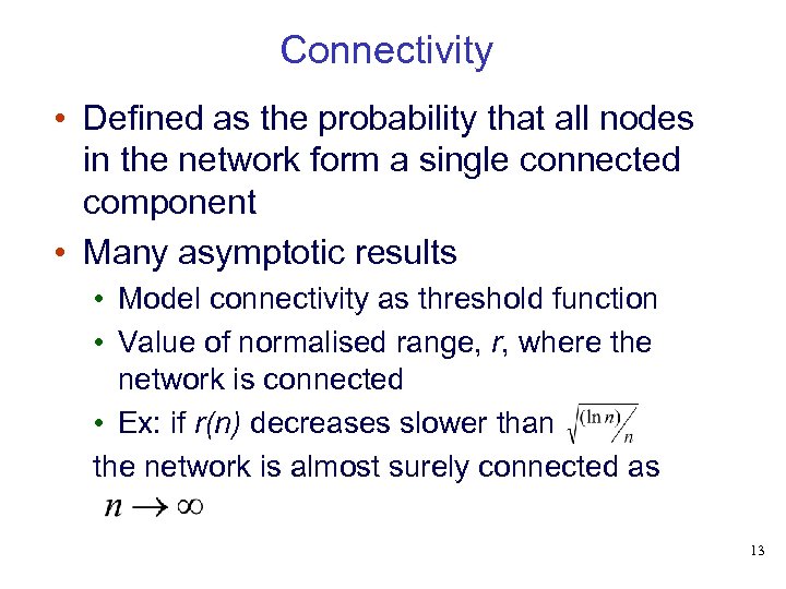Connectivity • Defined as the probability that all nodes in the network form a single connected component • Many asymptotic results • Model connectivity as threshold function • Value of normalised range, r, where the network is connected • Ex: if r(n) decreases slower than the network is almost surely connected as 13

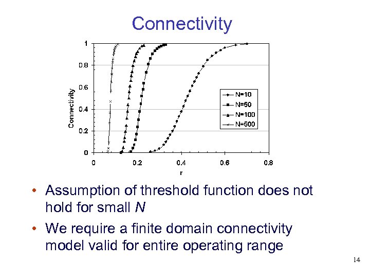Connectivity • Assumption of threshold function does not hold for small N • We require a finite domain connectivity model valid for entire operating range 14

Connectivity • Existing work in the finite domain • Exact expression for one-dimensional network [DM 02] • Empirical studies of k-connectivity [Kos 04] • Tang and others [TFL 03] • Empirical model of connectivity in twodimensions for N between 3 and 125 and connectivity between 0. 5 and 0. 99 • We present a more general and accurate empirical model 15

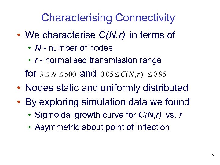Characterising Connectivity • We characterise C(N, r) in terms of • N - number of nodes • r - normalised transmission range for and • Nodes static and uniformly distributed • By exploring simulation data we found • Sigmoidal growth curve for C(N, r) vs. r • Asymmetric about point of inflection 16

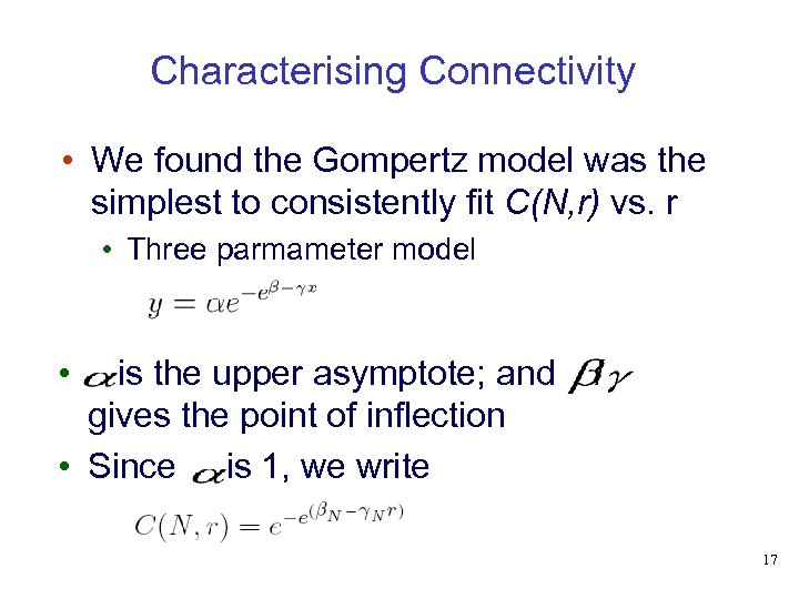Characterising Connectivity • We found the Gompertz model was the simplest to consistently fit C(N, r) vs. r • Three parmameter model • is the upper asymptote; and gives the point of inflection • Since is 1, we write / 17

Connectivity characterisation • 44 values of N between 2 and 500 • For each N, we conducted simulations to obtain r vs. C(N, r) values in the interval [0, 1] • Simulations with Simran • 10000 runs for each N, r value • Simulations accurate to within 0. 01 with 95% confidence 18

How many simulations? • The mean of n runs is known to have be within an error of where n is the number of samples and s is the standard deviation of the samples. • It can be shown that the largest value of s for connectivity experiments is 0. 5 • It follows that by using n > 9604 we can ensure error within 0. 01 with 95% confidence 19

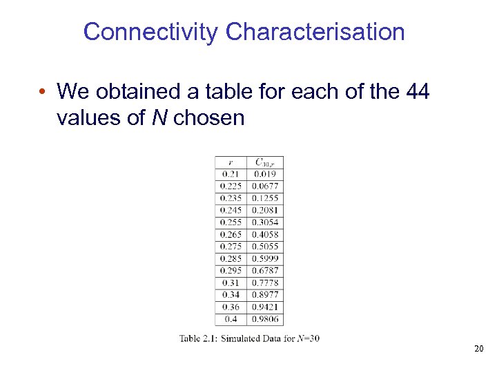Connectivity Characterisation • We obtained a table for each of the 44 values of N chosen 20

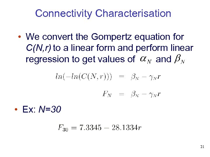Connectivity Characterisation • We convert the Gompertz equation for C(N, r) to a linear form and perform linear regression to get values of and • Ex: N=30 21

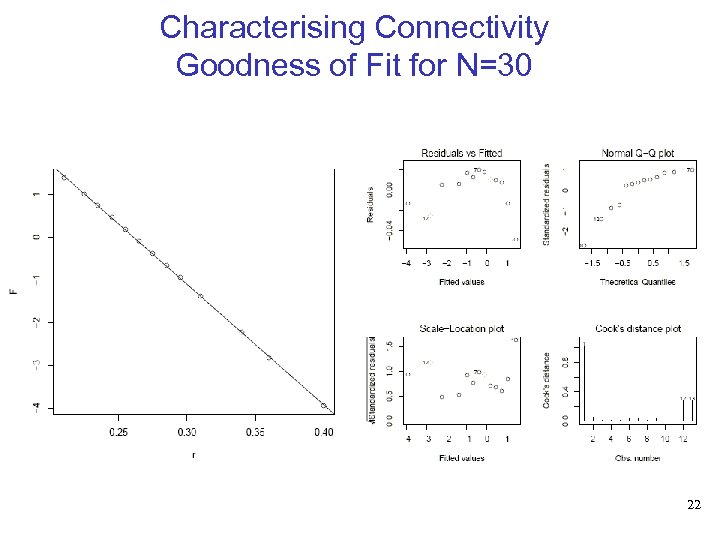Characterising Connectivity Goodness of Fit for N=30 22

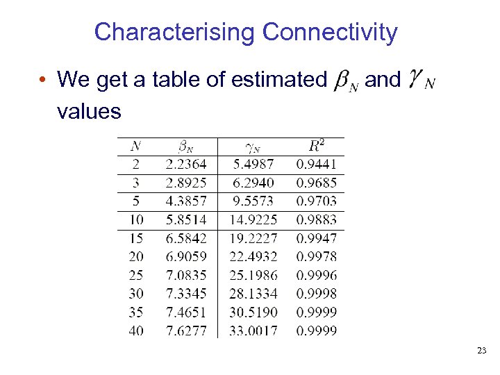Characterising Connectivity • We get a table of estimated values and 23

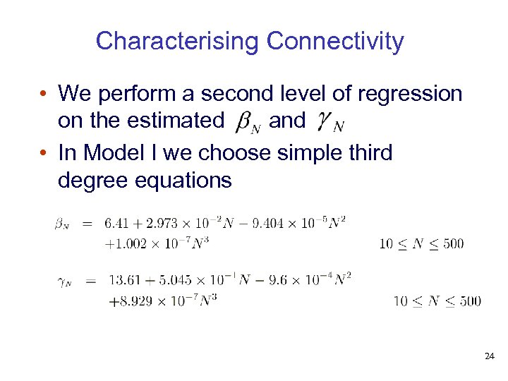Characterising Connectivity • We perform a second level of regression on the estimated and • In Model I we choose simple third degree equations 24

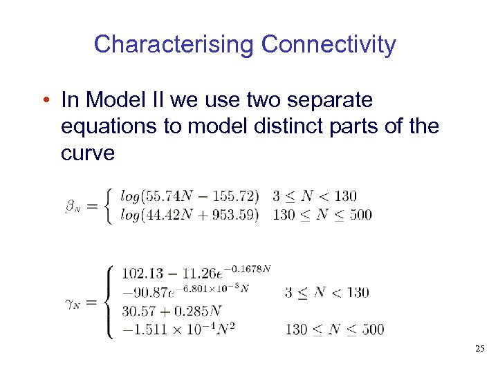Characterising Connectivity • In Model II we use two separate equations to model distinct parts of the curve 25

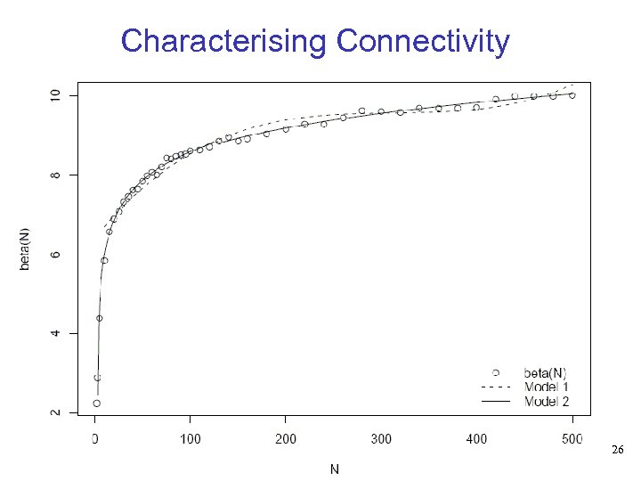Characterising Connectivity 26

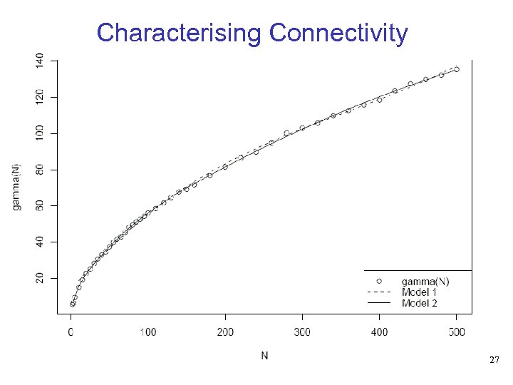Characterising Connectivity 27

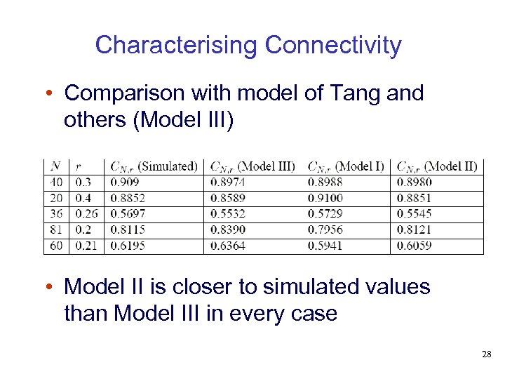Characterising Connectivity • Comparison with model of Tang and others (Model III) • Model II is closer to simulated values than Model III in every case 28

Characterising Connectivity - Validation • 236 N, r pairs • N's chosen don't contribute to model • r chosen to ensure connectivity value between 0. 05 and 0. 95 • 10000 simulations with the chosen N, r pairs compared with Models I and II • For Model I • N < 30: Mean absolute error 0. 069; maximum 0. 1756 • N > 30: mean absolute error of 0. 0116 with maximum seen being 0. 044 • For Model 2 • Mean absolute error of 0. 0089 with maximum of 0. 0418 29

Reachability 30

Connectivity in Sparse MWNs • May not be an indicator of actual extent to which network can support communication • Can be unresponsive to fine changes in network parameters • As an alternative, we propose that reachability has better properties for dealing with sparse networks 31

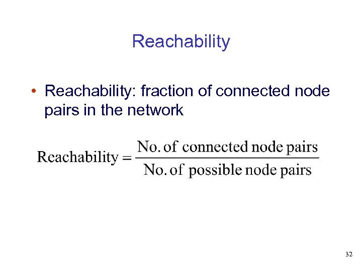Reachability • Reachability: fraction of connected node pairs in the network 32

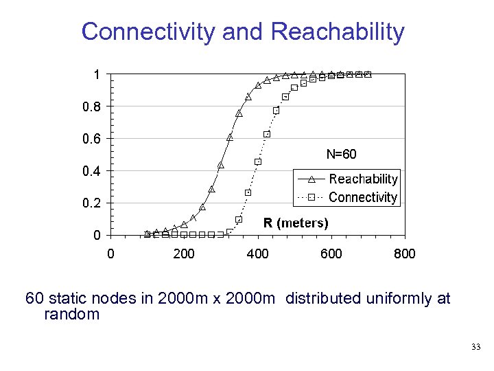Connectivity and Reachability 60 static nodes in 2000 m x 2000 m distributed uniformly at random 33

Connectivity and Reachability • When reachability is 0. 4 • 40% of node pairs are connected • But connectivity still at 0 • Connectivity remains at 0 from R = 50 to R = 320 m • Does not indicate actual extent of communication supported by the network • This gap increases with mobility and asynchronous communication 34

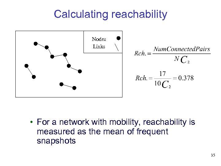Calculating reachability Nodes Links • For a network with mobility, reachability is measured as the mean of frequent snapshots 35

Properties of Reachability • Reachability: 1. lies in the interval [0, 1] 2. in a sparse network is not less than its connectivity 3. represents the probability that a randomly chosen pair of nodes in a network is connected 4. represents the long term maximal packet delivery ratio achievable between randomsource destination pairs in the network - Application: Normalised Packet Delivery Ratio 36

Case Study - Sparse multi-hop wireless for voice communication 37

Simulation study • Village spread across 2 km x 2 km • Low population density • Devices capable of multi-hop voice communication to be deployed • Simulations performed using Simran - a simulator for topological properties of wireless multi-hop networks 38

Choosing N If a certain device has R fixed at 300 m, how many nodes are needed to ensure that 60% of call attempts are successful? • Assumptions for simulations • Negligible mobility • Homogenous range assignment of R • Not a realistic propagation model • Results will be optimistic, but indicative • Average of 500 simulation results for each of several values of R 39

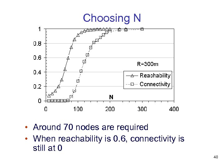Choosing N • Around 70 nodes are required • When reachability is 0. 6, connectivity is still at 0 40

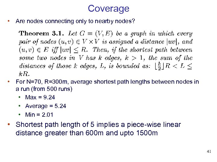Coverage • Are nodes connecting only to nearby nodes? • For N=70, R=300 m, average shortest path lengths between nodes in a run (from 500 runs) • Max = 9. 24 • Average = 5. 24 • Min = 2. 01 • Shortest path length of 5 implies a piece-wise linear distance greater than 600 m and upto 1500 m 41

Adding mobility • For the previous case, (N=70, R=300 m) we introduce mobility • Simulation time: 12 hours • Random way-point • Vmin=0. 5 ms-1 • Vmax=2 ms-1 • Pause = 30 mins • Reachability increases from 0. 6 to 0. 71 42

Asynchronous Communication • N=60, varying R • Uniform velocity of 5 ms-1 • Two nodes are connected at simulation time t if a path, possibly asynchronous, existed between them within time t+30 • That is, store-and-forward message passing can happen between the two nodes in 30 seconds • 20 simulations of 500 seconds each 43

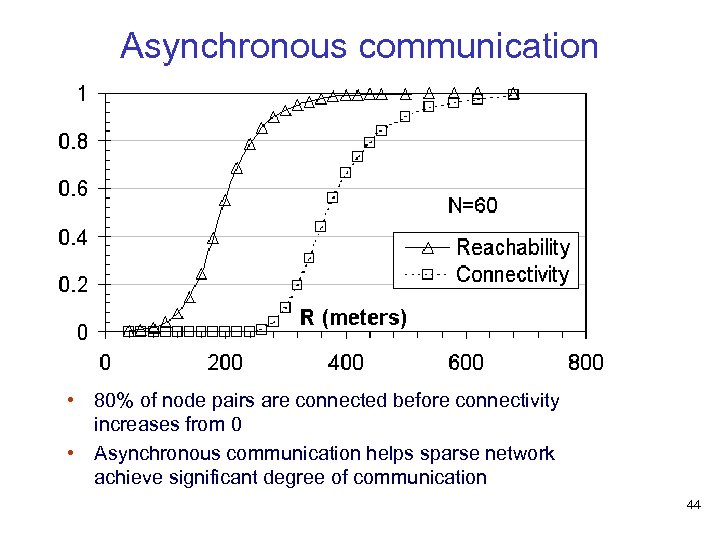Asynchronous communication • 80% of node pairs are connected before connectivity increases from 0 • Asynchronous communication helps sparse network achieve significant degree of communication 44

Characterising Reachability 45

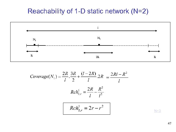
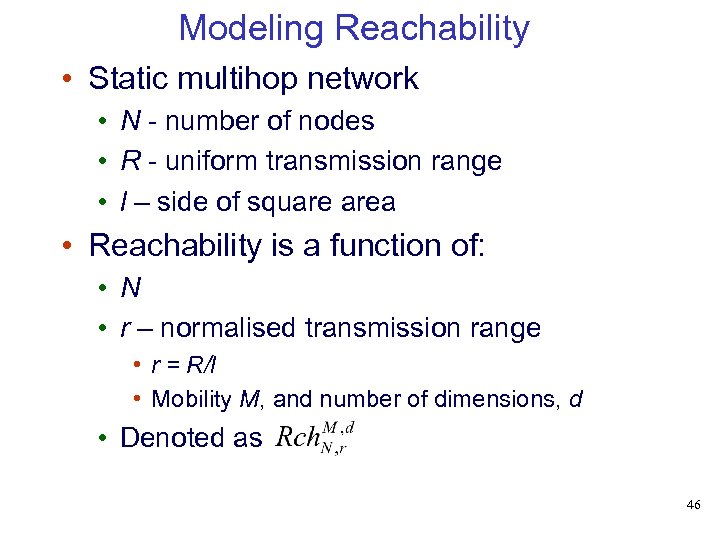Modeling Reachability • Static multihop network • N - number of nodes • R - uniform transmission range • l – side of square area • Reachability is a function of: • N • r – normalised transmission range • r = R/l • Mobility M, and number of dimensions, d • Denoted as 46

Reachability of 1 -D static network (N=2) l N 1 R N 1 2 R R N=3 47

Modeling Reachability • If N nodes form k components with mi nodes in the ith component: • Asymptotic bounds for Rch. N, r may be possible to derive • We are interested in finite domain results and we model Rch. N, r using regression on simulated data 48

Modeling Reachability • Observations from simulations indicate that reachability grows logistically • The logistic curve • Frequently used to model populations • Models rapid growth beyond a threshold up to a stable maximum 49

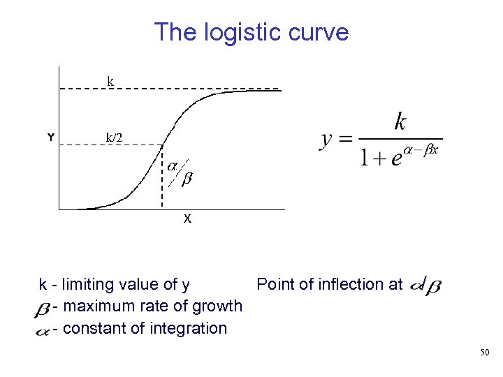The logistic curve k - limiting value of y Point of inflection at - maximum rate of growth - constant of integration / 50

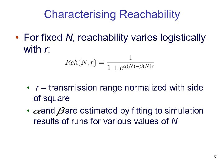Characterising Reachability • For fixed N, reachability varies logistically with r: • r – transmission range normalized with side of square • and are estimated by fitting to simulation results of runs for various values of N 51

Characterising Reachability • Simulations • 55 values of N between 2 and 500 • For each N, several values of r to span reachability from 0 to 1 • Each simulation run on 1000 randomly generated network graphs • Mean error within 0. 018 with 95% confidence • Yields a table of r vs. Rch(N, r) for one value of N 52

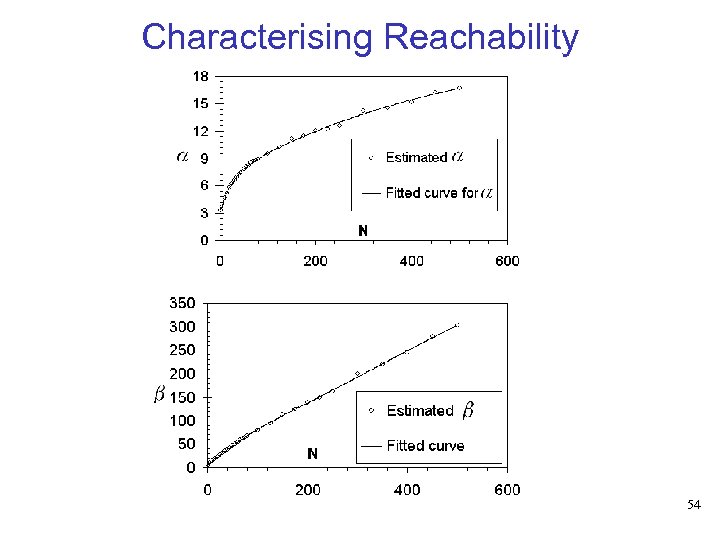
Characterising Reachability • and fitted in terms of N: • Average relative error around 3. 5% for cases that didn’t contribute to the model • Equations for and together with logistic equation characterize reachability • Model extended for N > 500 53

Characterising Reachability 54

Spanner • Design tool for sparse MWNs • Given three values from N, R, l and Rch, computes the fourth • Uses reachability model • Particularly useful for finding N • Cannot solve directly because functions of N • Binary search and are 55

Mobility • Our models for reachability and connectivity are most useful when nodes are mobile • Can be used with mobility models that retain uniform random distribution of nodes assumed in the model • Ex: Random direction [RMSM 01] 56

Edge effects on Connectivity Properties 57

Common assumptions in MWN topology design • Square or d-cube area of operation • Allows generalising results to 1 -, 2 -, and 3 -d • Toroidal area of operation • No edge effects to handle • Using node density as a parameter • Subsumes both N and area of operation 58

However… • Many practical deployment areas are rectangular • Connectivity properties are not geometry invariant • Two networks with similar nodes and equal node densities can have different values of connectivity • Significant in sparse networks 59

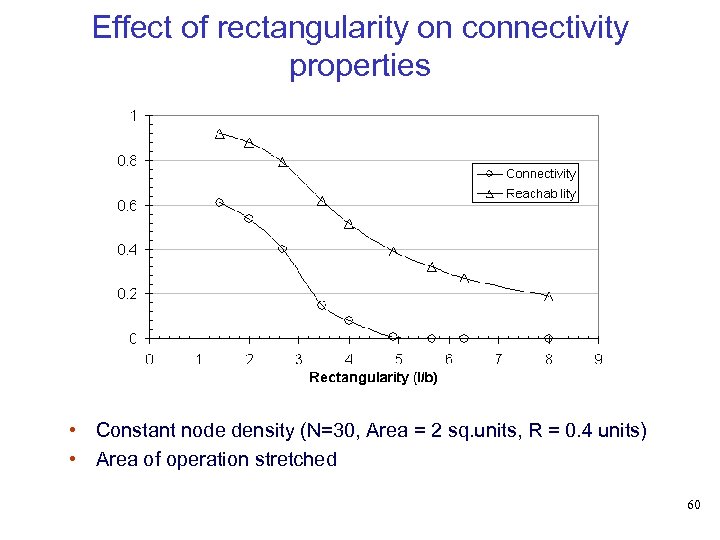Effect of rectangularity on connectivity properties • Constant node density (N=30, Area = 2 sq. units, R = 0. 4 units) • Area of operation stretched 60

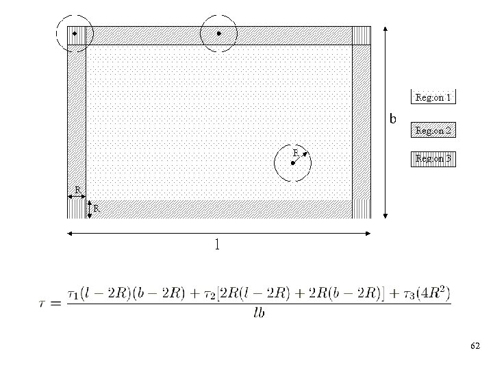
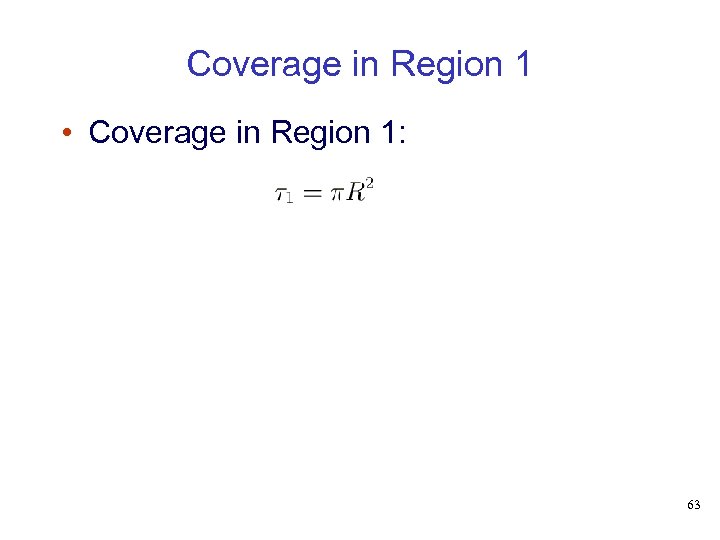
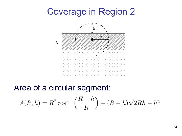
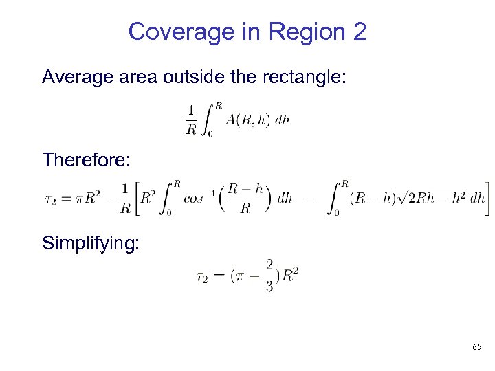
Edge effect • Part of transmission range not being used for connectivity • We define coverage as the effective transmission area of a node • Aim: • To determine exptected coverage, , for a single node with transmission range, R, in an l x b rectangle • To obtain an effective transmission range, Rlb to use with existing results for square areas 61

62

Coverage in Region 1 • Coverage in Region 1: 63

Coverage in Region 2 Area of a circular segment: 64

Coverage in Region 2 Average area outside the rectangle: Therefore: Simplifying: 65

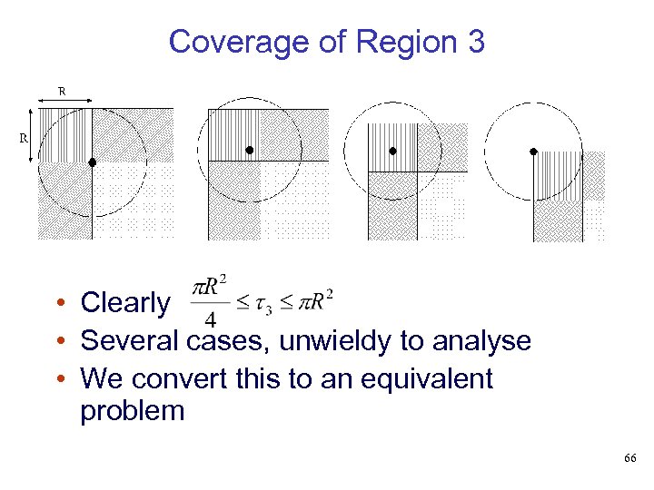Coverage of Region 3 • Clearly • Several cases, unwieldy to analyse • We convert this to an equivalent problem 66

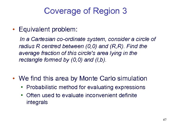Coverage of Region 3 • Equivalent problem: In a Cartesian co-ordinate system, consider a circle of radius R centred between (0, 0) and (R, R). Find the average fraction of this circle's area lying in the rectangle formed by (0, 0) and (l, b). • We find this area by Monte Carlo simulation • Probabilistic method for evaluating expressions • Often used to evaluate inconvenient definite integrals 67

Coverage of Region 3 • Run with: ; ; • We get: 68

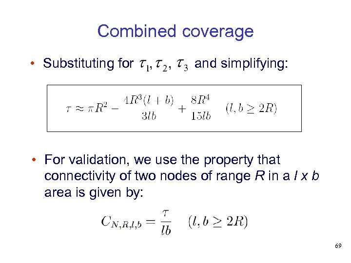Combined coverage • Substituting for , , and simplifying: • For validation, we use the property that connectivity of two nodes of range R in a l x b area is given by: 69

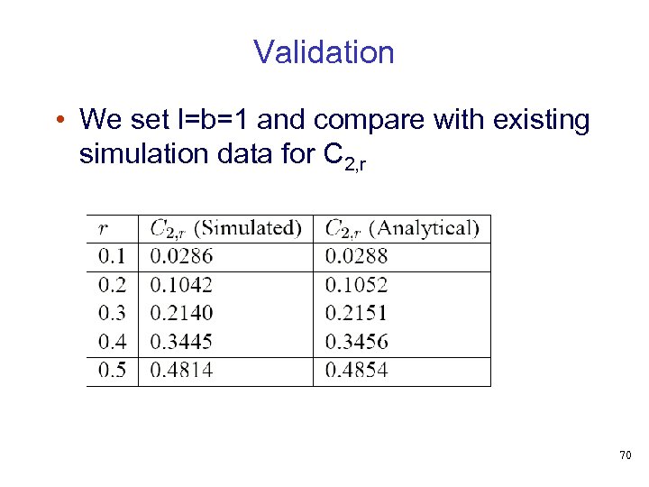Validation • We set l=b=1 and compare with existing simulation data for C 2, r 70

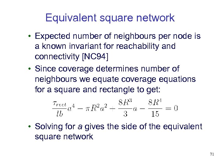Equivalent square network • Expected number of neighbours per node is a known invariant for reachability and connectivity [NC 94] • Since coverage determines number of neighbours we equate coverage equations for a square and rectangle to get: • Solving for a gives the side of the equivalent square network 71

Simran 72

Simran - Design Goals • Simran - simulator for topological simulations of MWNs • Support for metrics significant to design of sparse MWNs • Connectivity, reachability, size and number of connected components, average number of neighbours, shortest paths, etc. • Mobility support • Easy introduction of new mobility models • Support for asynchronous communication • Ease of running comparative simulations 73

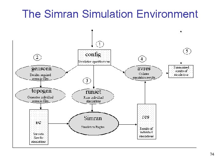The Simran Simulation Environment 74

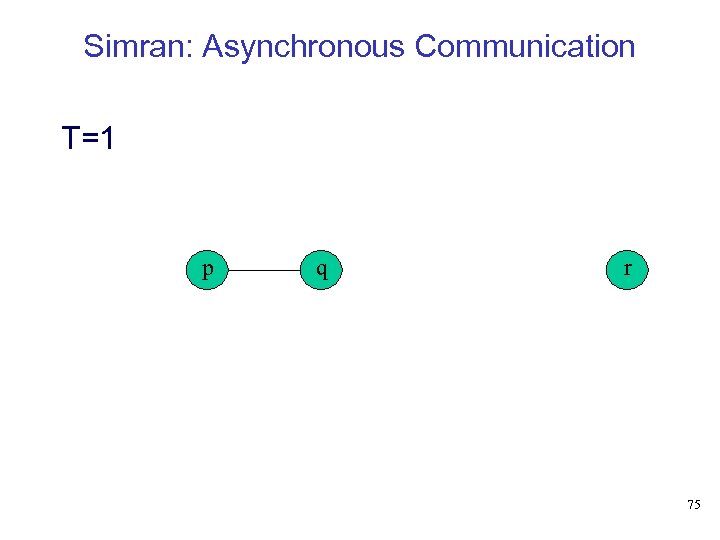Simran: Asynchronous Communication T=1 p q r 75

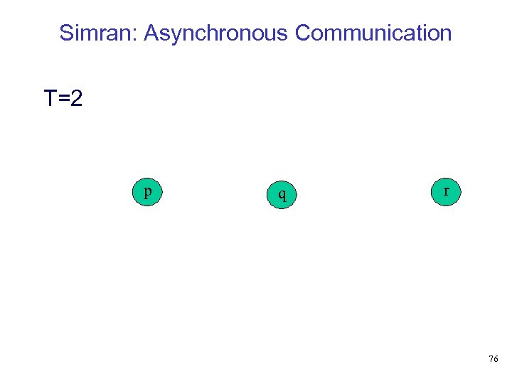Simran: Asynchronous Communication T=2 p q r 76

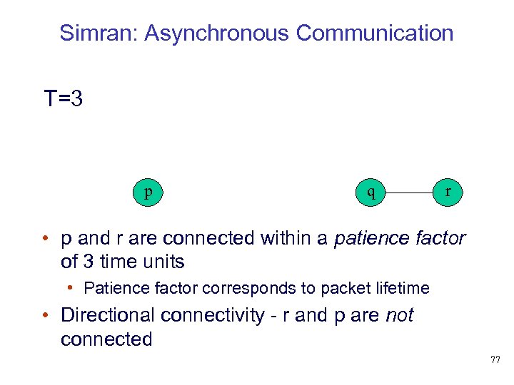Simran: Asynchronous Communication T=3 p q r • p and r are connected within a patience factor of 3 time units • Patience factor corresponds to packet lifetime • Directional connectivity - r and p are not connected 77

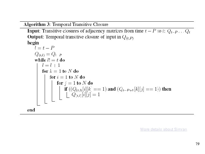
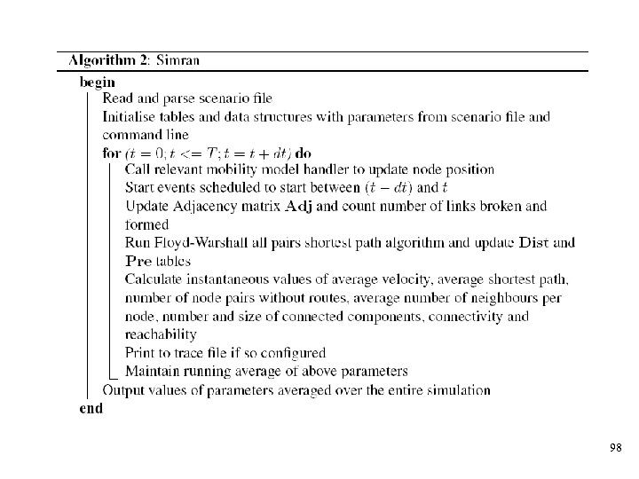
Simran: Temporal Transitive Closure (TTC) • Modification of Floyd-Warshall transitive closure algorithm • For a patience factor of P • Maintain sliding window of network state for last P-1 steps • Qt - transitive closure of adjacency matrix at present time, t • TTC - collapses Qt-p to Qt in into a single matrix in direction of time 78

More details about Simran 79

Conclusion 80

Contributions • Connectivity for sparse networks • Empirical, finite domain characterisation • Reachability • Definition and properties • Applications • Characterisation in the finite domain • Simran - a topological simulator for MWNs • Spanner - a design tool for sparse MWNs • Edge effects in MWNs • Quantifying the edge effect • Applying it to use results for square area networks in rectangular networks 81

Some future directions • Analytical models for reachability • Topology design in three dimensional networks • Are existing metrics sufficient? • Characterisations for 3 D networks • Models to interpret analytical results for deployment purposes • Simulation techniques • Realistic propagation models • Temporal network graph representations 82

Questions from Reviewer 1 1. Do you think this study could be applied to wireless sensor networks? If so, could you enumerate a few applications? If not, why? - It is applicable in any randomly deployed mobile sensor network. 2. Can you extend this work to coverage in WSNs where a sensor field does not have to be fully covered, i. e. , consider coverage instead of reachability? - This can be formulated as a problem in which discs of radii equal to the sensors' sensing range are dropped randomly to cover an area. It is very likely that the principle behind the usefulness of sparse networks is applicable here – it would be more economical if a small area left uncovered could be tolerated, and there could be a tradeoff between sensing range, number of sensors and covered area. An added factor of interest is a simultaneous requirement of some level of network communication. But it is not clear that our work can be directly extended to this problem. 83

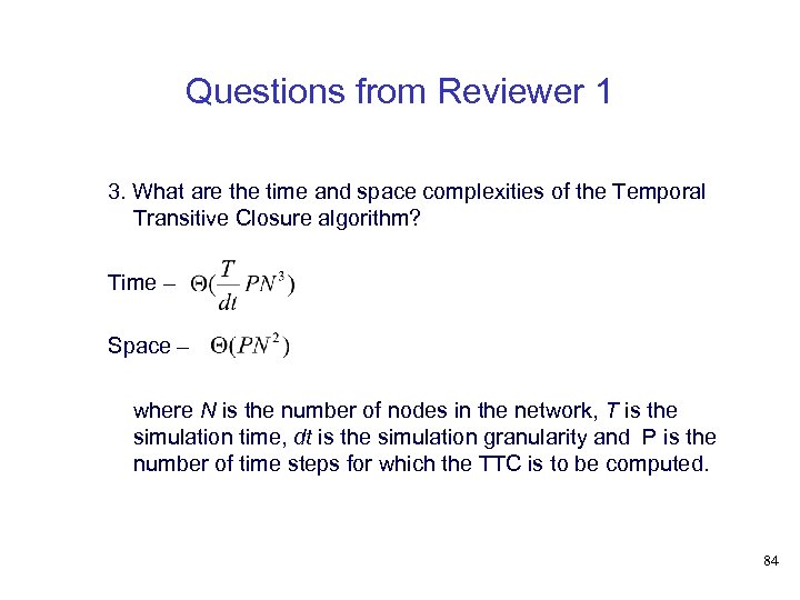Questions from Reviewer 1 3. What are the time and space complexities of the Temporal Transitive Closure algorithm? Time – Space – where N is the number of nodes in the network, T is the simulation time, dt is the simulation granularity and P is the number of time steps for which the TTC is to be computed. 84

Publications from the work presented (with Sridhar Iyer): • Characterization of a connectivity measure for sparse wireless multi-hop networks. Workshop on Wireless Ad hoc and Sensor Networks (WWASN), in conjunction with ICDCS, Lisboa, July 2006. (Expanded version appears in Ad Hoc and Sensor Wireless Networks Journal) • Designing sparse wireless multi-hop networks. Student workshop paper at IEEE INFOCOM, Barcelona, April 2006. • Reachability: An alternative to connectivity for sparse wireless multi-hop networks. Poster at IEEE INFOCOM, Barcelona, April 2006. • Sparse multi-hop wireless for voice communication in rural India. National Conference on Communications (NCC), New Delhi, January 2006. Other publications: • • Bridging the gap between reality and simulation: An Ethernet case study. (To appear) Conference on Information Technology (CIT), Bhubaneswar, December 2006. (With Punit Rathod and Raghuraman Rangarajan. ) Improving the performance of MANET routing protocols using cross-layer feedback. Conference on Information Technology (CIT), Bhubaneswar, December 2003. (With Leena Chandran-Wadia and Sridhar Iyer. ) Router handoff: A preemptive route repair strategy for AODV. IEEE International Conference on Personal Wireless Computing (IEEE ICPWC), New Delhi, December 2002. (With Abhilash P. and Sridhar Iyer. ) Router handoff: preemptive route repair in mobile ad hoc networks. International Conference on High Performance Computing (Hi. PC), Bangalore, December 2002. (With Abhilash P. and Sridhar Iyer. ) 85

Thank you 86

Supplementary slides 87

Normalised PDR for sparse networks • In a dense (unsaturated) network • Packet Delivery Ratio (PDR) measures the ability of the routing protocol to deliver packets to the intended destination • In a sparse network, PDR measures i. The network's ability to possess routes between nodes; and ii. The routing protocol's ability to exploit those routes 88

Normalised PDF for Sparse Networks • Using the property of Rch as maximal PDR, we can identify only the routing contribution by normalising PDR with reachability • NPDR = PDR/Rch • PDR value can be obtained from packet-level simulations or test-bed experiments • Rch for the network can be obtained from simulations or from a model Back to properties of reachability 89

Characterising Reachability • For larger values of N • Rch. N, r resembles a step function • Rch. N, r increase from 0. 1 to 0. 9 requires 0. 3 increase in r when N = 10, but only 0. 015 increase in r when N = 500 • Characterization is equivalent to finding the transition point, g. N. This is given by the point of inflection for the logistic curve 90

Characterising Reachability • Since the shape of and beta curves is relatively stable beyond N=200 • We estimate alpha and beta for N between 500 and 1000 by extrapolating from data points between 200 and 500: 91

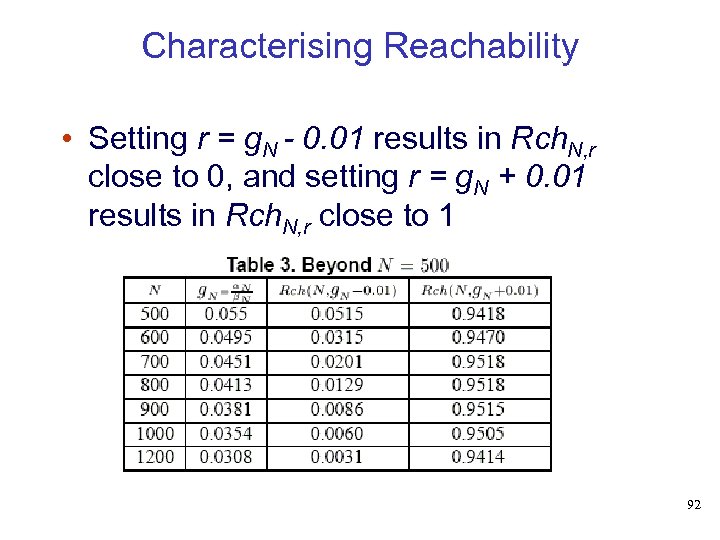Characterising Reachability • Setting r = g. N - 0. 01 results in Rch. N, r close to 0, and setting r = g. N + 0. 01 results in Rch. N, r close to 1 92

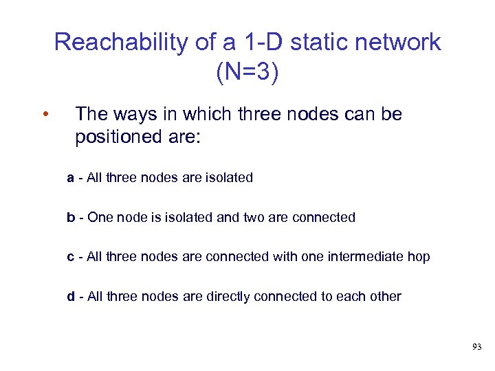Reachability of a 1 -D static network (N=3) • The ways in which three nodes can be positioned are: a - All three nodes are isolated b - One node is isolated and two are connected c - All three nodes are connected with one intermediate hop d - All three nodes are directly connected to each other 93

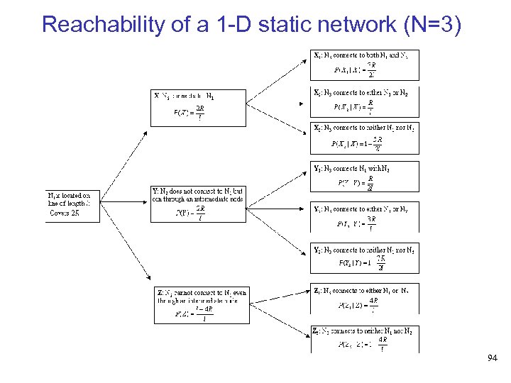Reachability of a 1 -D static network (N=3) 94

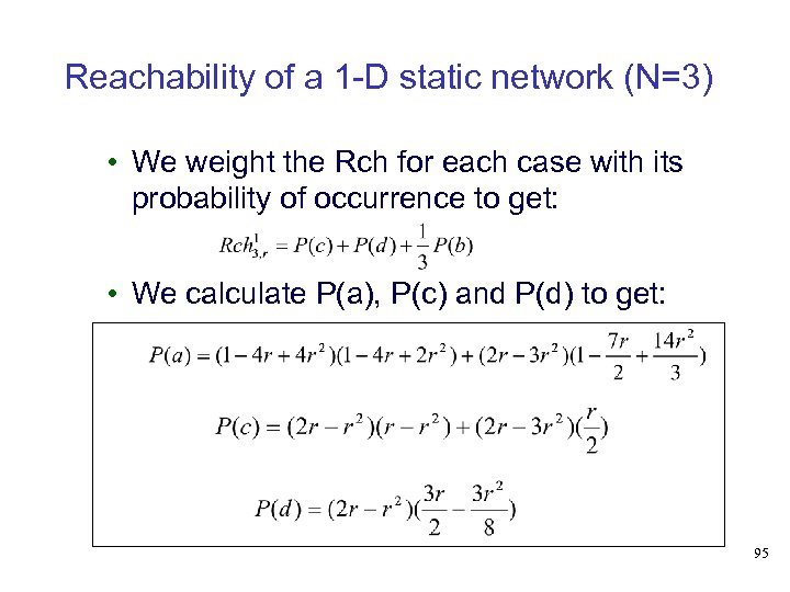Reachability of a 1 -D static network (N=3) • We weight the Rch for each case with its probability of occurrence to get: • We calculate P(a), P(c) and P(d) to get: 95

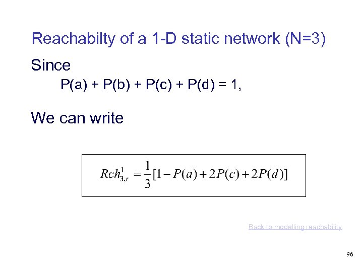Reachabilty of a 1 -D static network (N=3) Since P(a) + P(b) + P(c) + P(d) = 1, We can write Back to modelling reachability 96

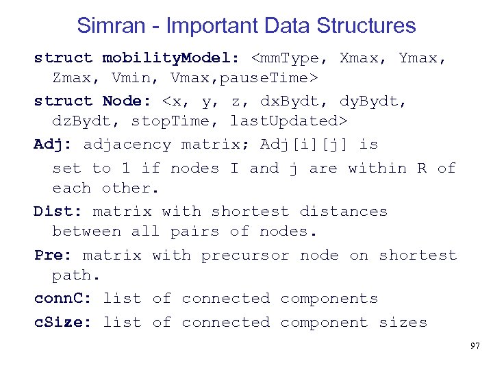Simran - Important Data Structures struct mobility. Model: struct Node: Adj: adjacency matrix; Adj[i][j] is set to 1 if nodes I and j are within R of each other. Dist: matrix with shortest distances between all pairs of nodes. Pre: matrix with precursor node on shortest path. conn. C: list of connected components c. Size: list of connected component sizes 97

98

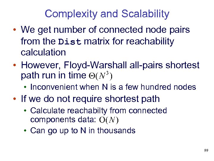Complexity and Scalability • We get number of connected node pairs from the Dist matrix for reachability calculation • However, Floyd-Warshall all-pairs shortest path run in time • Inconvenient when N is a few hundred nodes • If we do not require shortest path • Calculate reachabilty from connected components data: • Can go up to N in thousands 99

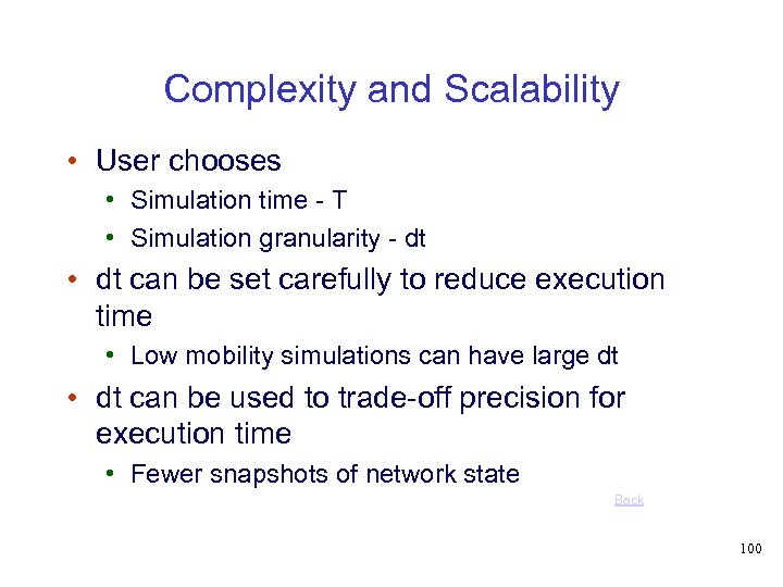Complexity and Scalability • User chooses • Simulation time - T • Simulation granularity - dt • dt can be set carefully to reduce execution time • Low mobility simulations can have large dt • dt can be used to trade-off precision for execution time • Fewer snapshots of network state Back 100