Conjoint and Discrete Choice Experiments DCEs Lecture

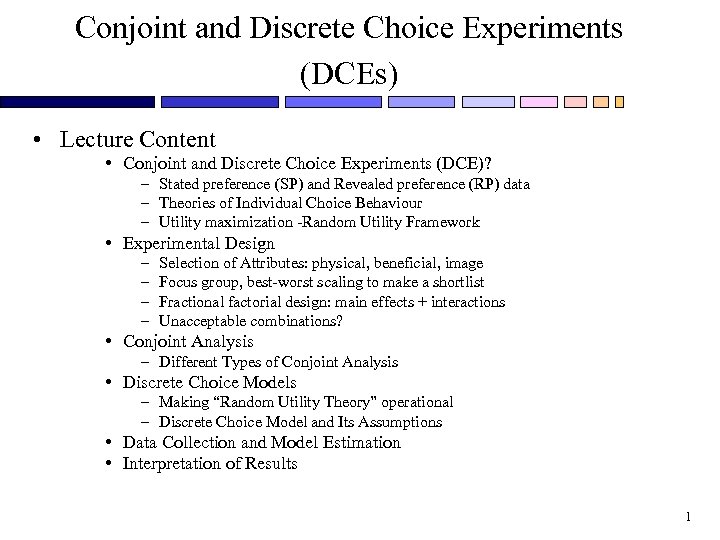Conjoint and Discrete Choice Experiments (DCEs) • Lecture Content • Conjoint and Discrete Choice Experiments (DCE)? – Stated preference (SP) and Revealed preference (RP) data – Theories of Individual Choice Behaviour – Utility maximization -Random Utility Framework • Experimental Design – – Selection of Attributes: physical, beneficial, image Focus group, best-worst scaling to make a shortlist Fractional factorial design: main effects + interactions Unacceptable combinations? • Conjoint Analysis – Different Types of Conjoint Analysis • Discrete Choice Models – Making “Random Utility Theory” operational – Discrete Choice Model and Its Assumptions • Data Collection and Model Estimation • Interpretation of Results 1

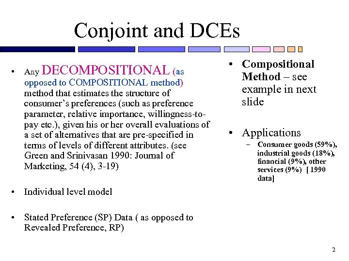Conjoint and DCEs • Any DECOMPOSITIONAL (as opposed to COMPOSITIONAL method) method that estimates the structure of consumer’s preferences (such as preference parameter, relative importance, willingness-topay etc. ), given his or her overall evaluations of a set of alternatives that are pre-specified in terms of levels of different attributes. (see Green and Srinivasan 1990: Journal of Marketing, 54 (4), 3 -19) • Compositional Method – see example in next slide • Applications – Consumer goods (59%), industrial goods (18%), financial (9%), other services (9%) [ 1990 data] • Individual level model • Stated Preference (SP) Data ( as opposed to Revealed Preference, RP) 2

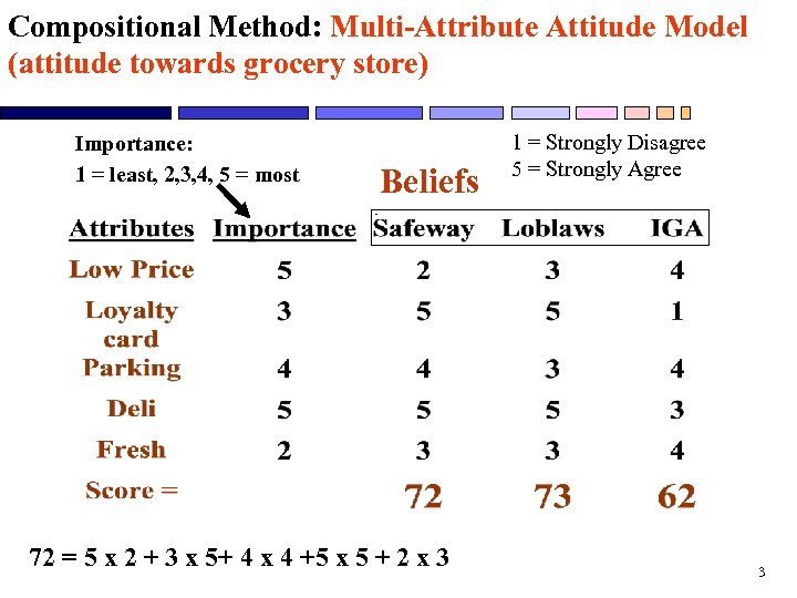Compositional Method: Multi-Attribute Attitude Model (attitude towards grocery store) Importance: 1 = least, 2, 3, 4, 5 = most Beliefs 72 = 5 x 2 + 3 x 5+ 4 x 4 +5 x 5 + 2 x 3 1 = Strongly Disagree 5 = Strongly Agree 3

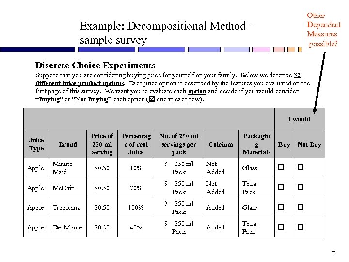Other Dependent Measures possible? Example: Decompositional Method – sample survey Discrete Choice Experiments Suppose that you are considering buying juice for yourself or your family. Below we describe 32 different juice product options. Each juice option is described by the features you evaluated on the first page of this survey. We want you to evaluate each option and decide if you would consider “Buying” or “Not Buying” each option ( one in each row). I would Juice Type Brand Price of 250 ml serving Percentag e of real Juice No. of 250 ml servings per pack Calcium Packagin g Materials Buy Not Buy Apple Minute Maid $0. 30 10% 3 – 250 ml Pack Not Added Glass Apple Mc. Cain $0. 50 70% 9 – 250 ml Pack Not Added Tetra. Pack Apple Tropicana $0. 50 100% 3 – 250 ml Pack Added Glass Apple Del Monte $0. 30 40% 9 – 250 ml Pack Added Tetra. Pack 4

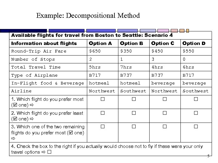Example: Decompositional Method Available flights for travel from Boston to Seattle: Scenario 4 Information about flights Option A Option B Option C Option D Round-Trip Air Fare $650 $350 $450 $550 Number of Stops 2 1 3 0 Total Travel Time 5 hrs 7 hrs 4 hrs 6 hrs Type of Airplane B 717 B 737 B 717 In-Flight food & Beverage hotmeal beverage Airline Northwest Southwest 1. Which flight do you prefer most ( one) 2. Which flight do you prefer least ( one) 3. Which one of the two remaining flights do you prefer most ( one) 4. Check the box to the right if you actually would choose not to fly if these were your only travel options 5

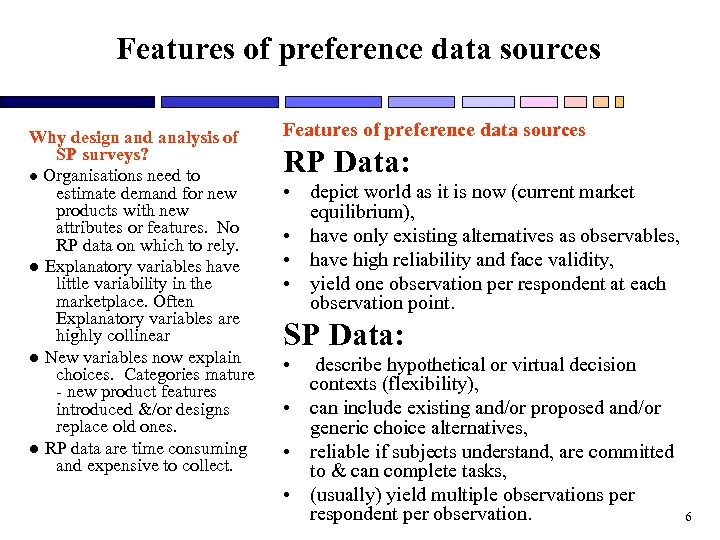Features of preference data sources Why design and analysis of SP surveys? ● Organisations need to estimate demand for new products with new attributes or features. No RP data on which to rely. ● Explanatory variables have little variability in the marketplace. Often Explanatory variables are highly collinear ● New variables now explain choices. Categories mature - new product features introduced &/or designs replace old ones. ● RP data are time consuming and expensive to collect. Features of preference data sources RP Data: • depict world as it is now (current market equilibrium), • have only existing alternatives as observables, • have high reliability and face validity, • yield one observation per respondent at each observation point. SP Data: • describe hypothetical or virtual decision contexts (flexibility), • can include existing and/or proposed and/or generic choice alternatives, • reliable if subjects understand, are committed to & can complete tasks, • (usually) yield multiple observations per respondent per observation. 6

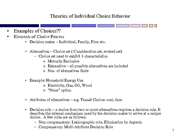Theories of Individual Choice Behavior • Examples of Choices? ? • Elements of Choice Process • Decision maker ~ Individual, Family, Firm etc. • Alternatives ~ Choice set ( Consideration set, evoked set) – Choice set need to exhibit 3 characteristics » Mutually Exclusive » Exhaustive – all possible alternatives are included » Nos. of alternatives finite • Example: Household Energy Use » Electricity, Gas, Oil, Wood » “None” option • Attributes of alternatives ~ e. g. Transit Choice: cost, time • Decision rule ~ a choice from two or more alternatives requires a decision rule. It describes the internal mechanism used by the decision maker to arrive at a unique choice. A few rules are as follows: – Non-compensatory: Lexicographic rule, Elimination by Aspects – Compensatory: Multi-Attribute Decision Rule 7

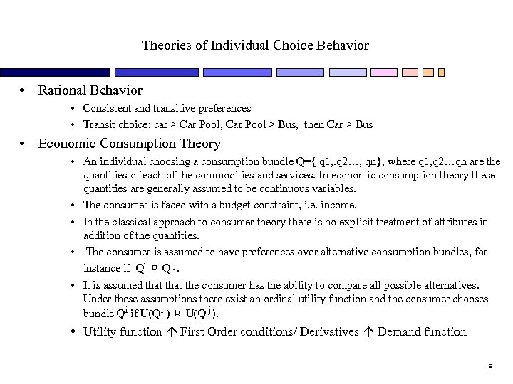Theories of Individual Choice Behavior • Rational Behavior • Consistent and transitive preferences • Transit choice: car > Car Pool, Car Pool > Bus, then Car > Bus • Economic Consumption Theory • An individual choosing a consumption bundle Q={ q 1, . q 2…, qn}, where q 1, q 2…qn are the quantities of each of the commodities and services. In economic consumption theory these quantities are generally assumed to be continuous variables. • The consumer is faced with a budget constraint, i. e. income. • In the classical approach to consumer theory there is no explicit treatment of attributes in addition of the quantities. • The consumer is assumed to have preferences over alternative consumption bundles, for instance if Qi Q j. • It is assumed that the consumer has the ability to compare all possible alternatives. Under these assumptions there exist an ordinal utility function and the consumer chooses bundle Qi if U(Qi ) U(Q j). • Utility function First Order conditions/ Derivatives Demand function 8

Theories of Individual Choice Behavior • Discrete Choice Theory • Transit Choice: Car Pool, Car, Bus, Train As we are dealing with a set of discrete choices, it is impossible to use the techniques used in “Economic Consumption Theory” (e. g. use of derivatives to derive demand function). Thus discrete choice problem requires a different analytical approach. We will retain the concept of “Rational Consumer” and concept of “Utility maximization”. Difference between “Choice Theory” and “Economic Consumption Theory”. – “Consumption theory” works with demand function derived from utility function but “Choice theory” work directly with the utility functions. • • • Random Utility Maximization – The approach of “Random Utility” is more in line with economic consumption theory and is theoretical behavioral approach for modeling choices. – The individual is always assumed to select the alternative with the highest utility. However, the utilities are not known to the analyst with certainty and are therefore treated by the analyst as random variables. – We are saying “Utility” is random. There a number of sources of “randomness” such as • unobserved attributes • unobserved taste variations • measurement errors and imperfect information – When Consumer will choose one alternative? 9

Discrete Choice Analysis: related • Variable Choice sets- in discrete choice experiments, we give respondents same choice sets (or consideration set). No of alternatives fixed. • Example: If consumer do not have car, then his/her alternatives are car pool, bus, and train. • Behavioral Theory- What if decision rule is “Noncompensatory” such as “Lexicographic” or “Elimination by Aspects”. This will lead to different choice model. Issues • Missing Information - What happens when we don’t give consumer full information i. e. choices under missing information. May influence “brand equity”, mean estimates, or variability. • Family Decision Making ( or interaction among households) • Current models are based on theory of individual decision making. Many decisions are based on the interactions of household members such as ‘home purchase 10

Experimental Design: Selection of Attributes • Wide variety of product attribute descriptions – mainly 3 types ( see Lefkoff- • • Beyond these utilitarian or functional benefits there is a stream of sociological work which consider symbolic aspects of product preferences • How product represent user to others or self-image Hagius and Mason (1993), 20 (1), 100 -110, Journal of Consumer Research): • (a) Characteristics / Physical properties / Tangible • Attributes that describes the physical properties • Physical attributes are objectively measured and meaningful to engineers and managers • (b) Beneficial / Functional / Intangible / Instrumental • What product will do to user • Economic theory suggests that consumers select products for the utility or benefit that they provide. Consumers want products not for physical products themselves but for the benefit derived from using the products (c) Image / Intangible/ abstract • Possibility of correlations among 3 types of attributes • Physical characteristics are often causally linked to beneficial attributes. – presence of air bag, antilock brakes determines safety of a car. • Correlation between beneficial and image attributes – Fast acceleration, tight cornering projects sporty image 11

Experimental Design: Selection of Attributes Designs Science of planning exactly what observations to take and how to take them to permit the best possible inferences to be made from data vis-à-vis one’s hypothesis. Designed experiments manipulate attributes and levels to permit rigorous tests of certain hypothesis of interest Experiment manipulates one or more attributes • Attribute list – Also called “factors”, “explanatory variables”, “independent variables”, “features” etc – Make list of attributes – from previous surveys, consumers, experts – Make a short list of attributes – focus group, bestworst scaling – Check for conceptual correlation between the attributes • Identify attribute levels – experiment with one attribute • each level is called TREATMENT – Experiment with more than one attribute • Each unique combination of factor levels is called “TREATMENT COMBINATION” – Marketers call this treatment combination “PROFILES” 12

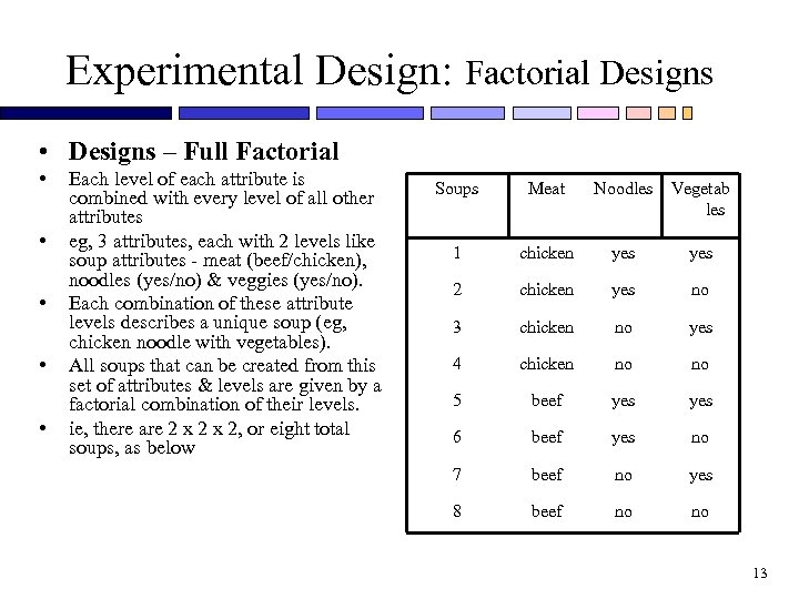Experimental Design: Factorial Designs • Designs – Full Factorial • • • Each level of each attribute is combined with every level of all other attributes eg, 3 attributes, each with 2 levels like soup attributes - meat (beef/chicken), noodles (yes/no) & veggies (yes/no). Each combination of these attribute levels describes a unique soup (eg, chicken noodle with vegetables). All soups that can be created from this set of attributes & levels are given by a factorial combination of their levels. ie, there are 2 x 2, or eight total soups, as below Soups Meat Noodles Vegetab les 1 chicken yes 2 chicken yes no 3 chicken no yes 4 chicken no no 5 beef yes 6 beef yes no 7 beef no yes 8 beef no no 13

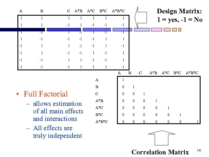A B C A*B A*C B*C 1 1 1 1 1 -1 -1 -1 1 -1 -1 1 -1 -1 1 -1 -1 -1 1 Design Matrix: 1 = yes, -1 = No A*B*C -1 A B C A*B A*C B*C A • Full Factorial – allows estimation of all main effects and interactions – All effects are truly independent 1 B 0 1 C 0 0 1 A*B 0 0 0 1 A*C 0 0 1 B*C 0 0 0 1 A*B*C 0 0 0 A*B*C 0 Correlation Matrix 1 14

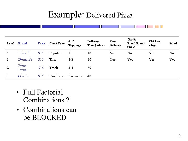Example: Delivered Pizza Delivery Time (mins. ) Free Delivery Garlic Bread/Bread Sticks Chicken wings Salad Level Brand Price Crust Type # of Toppings 0 Pizza Hut $10 Regular 1 10 No No 1 Domino's $12 Thin 2 -3 20 Yes Yes 2 Pizza $14 Thick 4 -5 30 3 Gino's $16 Pan pizza 6 or more 40 • Full Factorial Combinations ? • Combinations can be BLOCKED 15

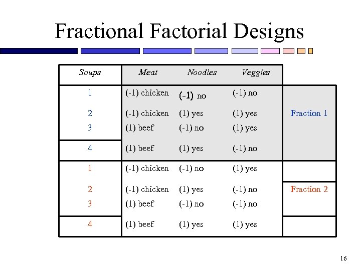Fractional Factorial Designs Soups Meat Noodles Veggies 1 (-1) chicken (-1) no 2 (-1) chicken (1) yes 3 (1) beef (-1) no (1) yes 4 (1) beef (1) yes (-1) no 1 (-1) chicken (-1) no (1) yes 2 (-1) chicken (1) yes (-1) no 3 (1) beef (-1) no 4 (1) beef (1) yes Fraction 1 Fraction 2 16

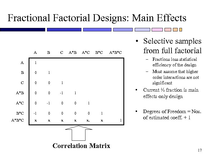Fractional Factorial Designs: Main Effects A B C A*B A*C B*C A*B*C • Selective samples from full factorial – Fractions loss statistical efficiency of the design – Must assume that higher order interactions are not significant A 1 B 0 1 C 0 0 1 A*B 0 0 -1 1 A*C 0 -1 0 0 1 B*C -1 0 0 1 A*B*C x x x. x • Correlation Matrix • 1 Current ½ fraction is main effects only design Degrees of Freedom = Nos. of estimated coeff. + 1 17

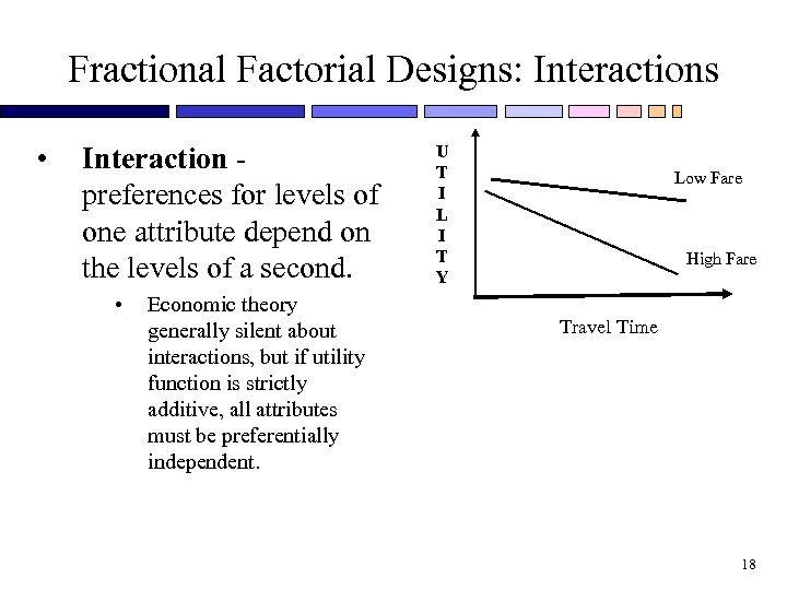Fractional Factorial Designs: Interactions • Interaction preferences for levels of one attribute depend on the levels of a second. • Economic theory generally silent about interactions, but if utility function is strictly additive, all attributes must be preferentially independent. U T I L I T Y Low Fare High Fare Travel Time 18

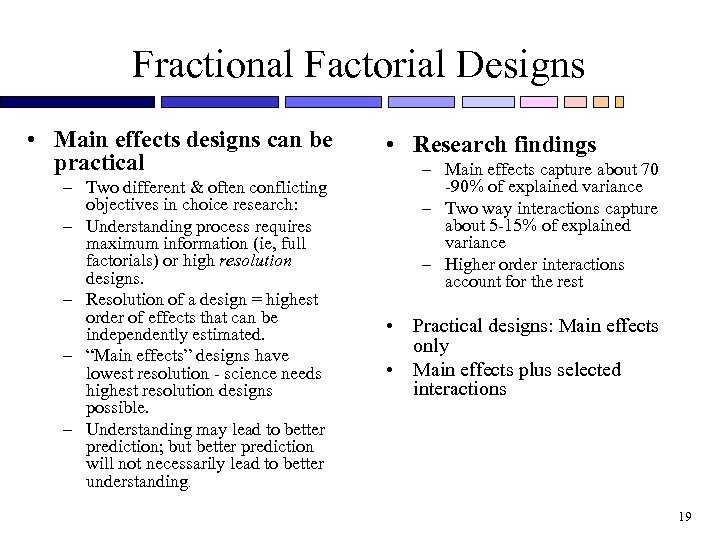Fractional Factorial Designs • Main effects designs can be practical – Two different & often conflicting objectives in choice research: – Understanding process requires maximum information (ie, full factorials) or high resolution designs. – Resolution of a design = highest order of effects that can be independently estimated. – “Main effects” designs have lowest resolution - science needs highest resolution designs possible. – Understanding may lead to better prediction; but better prediction will not necessarily lead to better understanding. • Research findings – Main effects capture about 70 -90% of explained variance – Two way interactions capture about 5 -15% of explained variance – Higher order interactions account for the rest • Practical designs: Main effects only • Main effects plus selected interactions 19

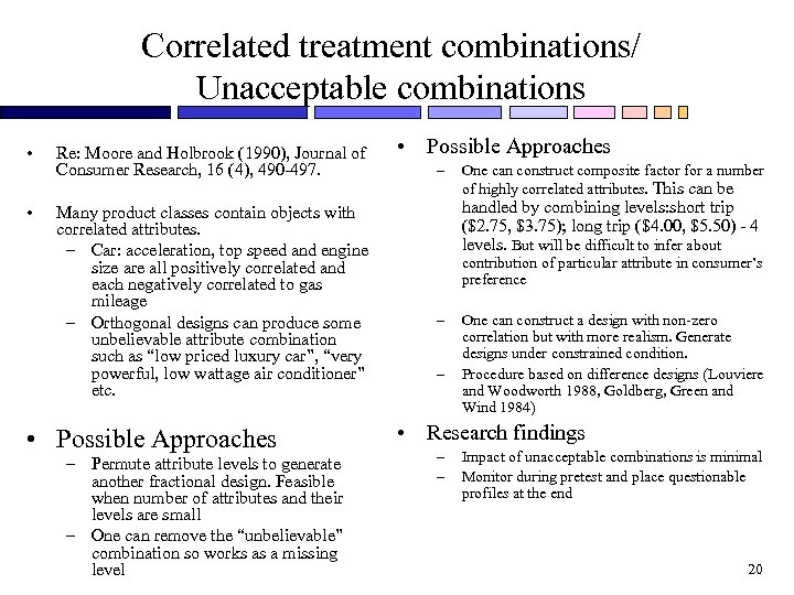Correlated treatment combinations/ Unacceptable combinations • Re: Moore and Holbrook (1990), Journal of Consumer Research, 16 (4), 490 -497. • Many product classes contain objects with correlated attributes. – Car: acceleration, top speed and engine size are all positively correlated and each negatively correlated to gas mileage – Orthogonal designs can produce some unbelievable attribute combination such as “low priced luxury car”, “very powerful, low wattage air conditioner” etc. • Possible Approaches – Permute attribute levels to generate another fractional design. Feasible when number of attributes and their levels are small – One can remove the “unbelievable” combination so works as a missing level • Possible Approaches – One can construct composite factor for a number of highly correlated attributes. This can be handled by combining levels: short trip ($2. 75, $3. 75); long trip ($4. 00, $5. 50) - 4 levels. But will be difficult to infer about contribution of particular attribute in consumer’s preference – – One can construct a design with non-zero correlation but with more realism. Generate designs under constrained condition. Procedure based on difference designs (Louviere and Woodworth 1988, Goldberg, Green and Wind 1984) • Research findings – – Impact of unacceptable combinations is minimal Monitor during pretest and place questionable profiles at the end 20

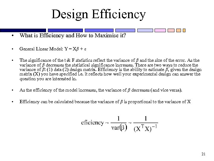Design Efficiency • What is Efficiency and How to Maximise it? • General Linear Model: Y = Xβ + ε • The significance of the t & F statistics reflect the variance of β and the size of the error. As the variance of β decreases the statistical significance increases. There are two ways to reduce the variance of β: (1) data (2) design matrix. Efficiency is the ability to estimate β, given the design matrix (X) you have specified i. e. it reflects how well your experimental design can answer the question you are interested in. • As the efficiency of the model increases, the variance of β decreases (and vice versa). • Efficiency can be calculated because the variance of β is proportional to the variance of X 21

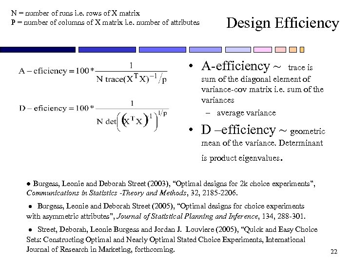N = number of runs i. e. rows of X matrix P = number of columns of X matrix i. e. number of attributes Design Efficiency • A-efficiency ~ trace is sum of the diagonal element of variance-cov matrix i. e. sum of the variances – average variance • D –efficiency ~ geometric mean of the variance. Determinant is product eigenvalues. ● Burgess, Leonie and Deborah Street (2003), “Optimal designs for 2 k choice experiments”, Communications in Statistics -Theory and Methods, 32, 2185 -2206. ● Burgess, Leonie and Deborah Street (2005), “Optimal designs for choice experiments with asymmetric attributes”, Journal of Statistical Planning and Inference, 134, 288 -301. ● Street, Deborah, Leonie Burgess and Jordan J. Louviere (2005), “Quick and Easy Choice Sets: Constructing Optimal and Nearly Optimal Stated Choice Experiments, International Journal of Research in Marketing, forthcoming. 22

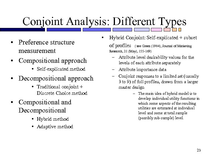Conjoint Analysis: Different Types • Preference structure measurement • Compositional approach • Self-explicated method • Decompositional approach • Traditional conjoint + Discrete Choice method • Compositional and Decompositional • Hybrid method • Adaptive method • Hybrid Conjoint: Self-explicated + subset of profiles ( see Green (1984), Journal of Marketing Research, 21 (May), 155 -169) – Attribute level desirability values for the levels of each attribute separately – Attribute importance data – Conjoint responses to a limited set (usually 3 to 9) of full profiles, drawn from a larger master design – The main idea of hybrid model is to develop individual utility functions in which some aspects of the resulting utilities are estimated at individual level and some at total sample (possibly sub-sample) level. 23

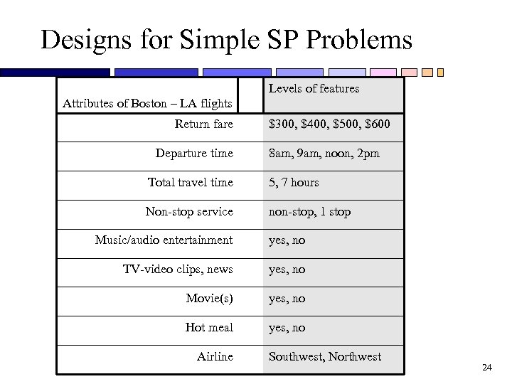Designs for Simple SP Problems Levels of features Attributes of Boston – LA flights Return fare Departure time $300, $400, $500, $600 8 am, 9 am, noon, 2 pm Total travel time 5, 7 hours Non-stop service non-stop, 1 stop Music/audio entertainment yes, no TV-video clips, news yes, no Movie(s) yes, no Hot meal yes, no Airline Southwest, Northwest 24

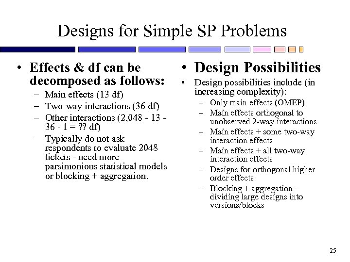Designs for Simple SP Problems • Effects & df can be decomposed as follows: – Main effects (13 df) – Two-way interactions (36 df) – Other interactions (2, 048 - 13 36 - 1 = ? ? df) – Typically do not ask respondents to evaluate 2048 tickets - need more parsimonious statistical models or blocking + aggregation. • Design Possibilities • Design possibilities include (in increasing complexity): – Only main effects (OMEP) – Main effects orthogonal to unobserved 2 -way interactions – Main effects + some two-way interaction effects – Main effects + all two-way interaction effects – Designs for orthogonal higher order effects – Blocking + aggregation – dividing large designs into versions/blocks 25

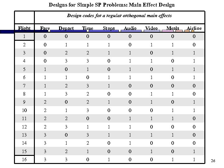Designs for Simple SP Problems: Main Effect Design codes for a regular orthogonal main effects Flight Fare Depart Time Stops Audio Video Meals Airline 1 0 0 0 0 2 0 1 1 1 0 3 0 2 2 1 1 0 1 1 4 0 3 3 0 1 1 0 1 5 1 0 1 0 1 1 6 1 1 0 1 7 1 2 3 1 0 0 8 1 3 2 0 0 1 1 0 9 2 0 2 1 0 1 10 2 1 3 0 0 0 1 1 11 2 2 0 0 1 1 1 0 12 2 3 1 1 1 0 0 0 13 3 0 3 1 1 0 14 3 1 2 0 1 0 0 0 15 3 2 1 0 0 1 16 3 3 0 1 0 0 1 1 26

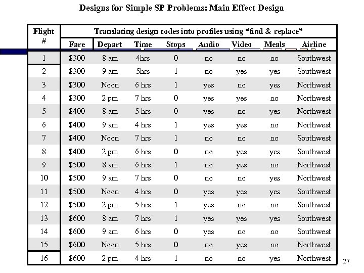Designs for Simple SP Problems: Main Effect Design Flight # Translating design codes into profiles using “find & replace” Fare Depart Time Stops Audio Video Meals Airline 1 $300 8 am 4 hrs 0 no no no Southwest 2 $300 9 am 5 hrs 1 no yes Southwest 3 $300 Noon 6 hrs 1 yes no yes Northwest 4 $300 2 pm 7 hrs 0 yes no Northwest 5 $400 8 am 5 hrs 0 yes no yes Northwest 6 $400 9 am 4 hrs 1 yes no Northwest 7 $400 Noon 7 hrs 1 no no no Southwest 8 $400 2 pm 6 hrs 0 no yes Southwest 9 $500 8 am 6 hrs 1 no yes no Northwest 10 $500 9 am 7 hrs 0 no no yes Northwest 11 $500 Noon 4 hrs 0 yes yes Southwest 12 $500 2 pm 5 hrs 1 yes no no Southwest 13 $600 8 am 7 hrs 1 yes yes Southwest 14 $600 9 am 6 hrs 0 yes no no Southwest 15 $600 Noon 5 hrs 0 no yes no Northwest 16 $600 2 pm 4 hrs 1 no no yes Northwest 27

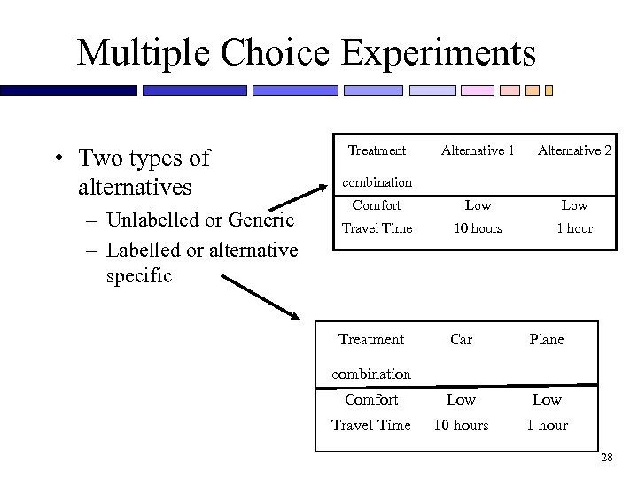Multiple Choice Experiments • Two types of alternatives – Unlabelled or Generic – Labelled or alternative specific Treatment Alternative 1 Alternative 2 Comfort Low Travel Time 10 hours 1 hour Treatment Car Plane Comfort Low Travel Time 10 hours 1 hour combination 28

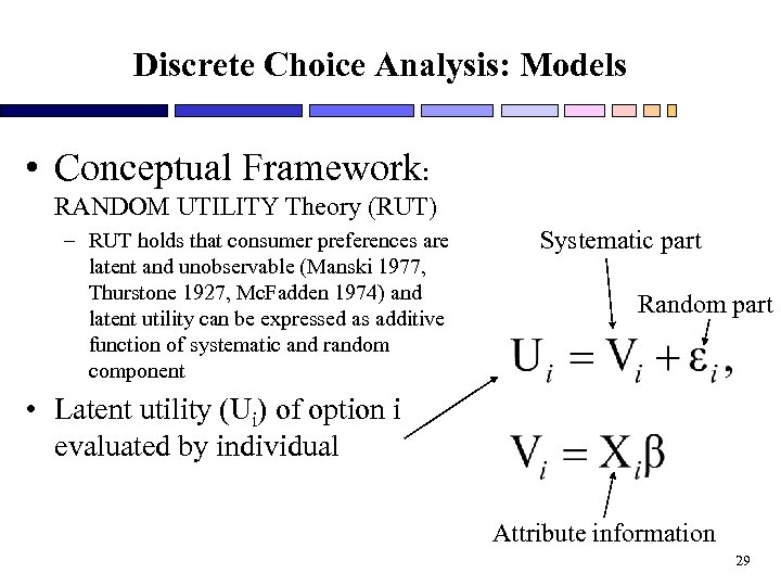Discrete Choice Analysis: Models • Conceptual Framework: RANDOM UTILITY Theory (RUT) – RUT holds that consumer preferences are latent and unobservable (Manski 1977, Thurstone 1927, Mc. Fadden 1974) and latent utility can be expressed as additive function of systematic and random component Systematic part Random part • Latent utility (Ui) of option i evaluated by individual Attribute information 29

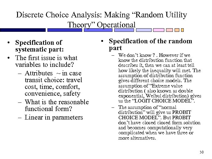Discrete Choice Analysis: Making “Random Utility Theory” Operational • Specification of systematic part: • The first issue is what variables to include? – Attributes ~ in case transit choice: travel cost, time, comfort, convenience, safety – What is the reasonable functional form? – Linear in parameters • Specification of the random part – We don’t know ? . However if we know the distribution function that describes it, then we can at least tell how likely the inequality will met. The assumption of distribution function gives different choice models. The assumption of “Extreme value distribution ( also known as double exponential, Weibul distribution) gives us the “LOGIT CHOICE MODEL”. – The assumption of “normal distribution” will give us PROBIT CHOICE MODEL”. But PROBIT don’t have closed form solution and becomes computationally very complicated when we have three or more alternatives. 30

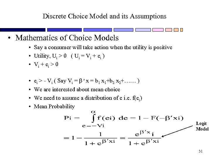Discrete Choice Model and its Assumptions • Mathematics of Choice Models • Say a consumer will take action when the utility is positive • Utility, Ui > 0 ( Ui = Vi + ei ) • Vi + e i > 0 • • ei > - Vi ( Say Vi = 'x = b 1 x 1+b 2 x 2+…… ) We are interested about mean choice We need to assume a distribution of e i. e. f(ei) Mean Probability Logit Model 31

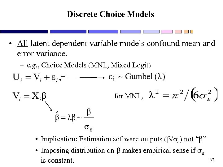Discrete Choice Models • All latent dependent variable models confound mean and error variance. – e. g. , Choice Models (MNL, Mixed Logit) for MNL, • Implication: Estimation software outputs ( / ) not “ ” • Imposing distribution on makes empirical sense if is constant. 32

Binary Choice Model Binary Choice: P(yes|yes, no) = exp(Vyes)/[exp(Vyes) + exp(Vno)], Vno can be set = 0 to satisfy the identification restriction. Thus, P(yes|yes, no) = exp(Vyes)/[exp(Vyes) + 1], The odds of responding “yes” relative to “no” are Taking natural logarithms of both sides, we see that: Vyes specified as linear-in-parameters: Vyes = k k. Xk + m m. Zm, k - vector of K attribute effects (Xk); m - vector of M individual measure effects (Zm) interacteed with intercept or elements of Xk. Key property – can effects of Xk be estimated independently? Xk contains main effects + (possibly) interactions - so, models that can be estimated depend on design of Xk columns. 33

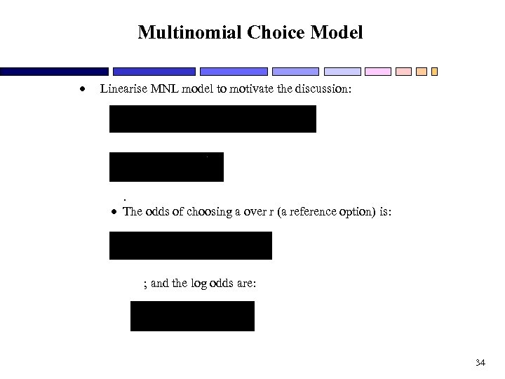Multinomial Choice Model Linearise MNL model to motivate the discussion: or, . The odds of choosing a over r (a reference option) is: ; and the log odds are: 34

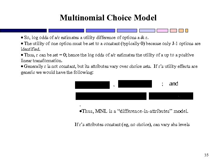Multinomial Choice Model So, log odds of a/r estimates a utility difference of options a & r. The utility of one option must be set to a constant (typically 0) because only J-1 options are identified. Thus, r can be set = 0; hence the log odds of a/r estimates the utility of a up to a positive linear transformation. Generally r is not constant, but its attributes vary over choice sets. If r’s utility effects are generic we would have the following: , ; and . Thus, MNL is a “difference-in-attributes” model. If r’s attributes constant (eg, no choice), can vary abs levels 35

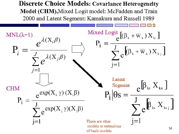Discrete Choice Models: Covariance Heterogeneity Model (CHM), Mixed Logit model: Mc. Fadden and Train 2000 and Latent Segment: Kamakura and Russell 1989 MNL(λ=1) CHM Mixed Logit Latent Segment There are other models or extensions of basic models 36

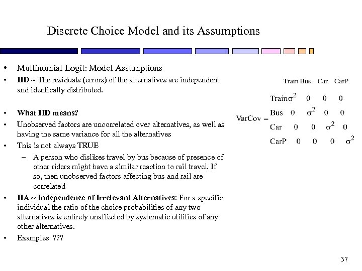Discrete Choice Model and its Assumptions • Multinomial Logit: Model Assumptions • IID ~ The residuals (errors) of the alternatives are independent and identically distributed. • • What IID means? Unobserved factors are uncorrelated over alternatives, as well as having the same variance for all the alternatives This is not always TRUE – A person who dislikes travel by bus because of presence of other riders might have a similar reaction to rail travel. If so, then unobserved factors affecting bus and rail are correlated IIA ~ Independence of Irrelevant Alternatives: For a specific individual the ratio of the choice probabilities of any two alternatives is entirely unaffected by systematic utilities of any other alternatives. Examples ? ? ? • • • 37

Data Collection and Estimation • Calculation of Sample size and sampling • Design • Convert design into Survey • Presentation format – mail, interview, online, computerassisted • Generate sample design using SPSS • Generate sample design using SAS 38

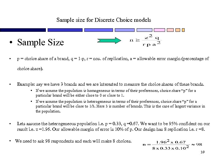Sample size for Discrete Choice models • Sample Size • p = choice share of a brand, q = 1 -p, r = nos. of replication, a = allowable error margin (percentage of choice share). • Example: say we have 3 brands and we are interested to measure the choice shares of these brands. • If we assume the population is homogeneous in terms of their preferences, choice share “p” for a particular brand will be either close to 0 or close to 1. • If we assume the population is heterogeneous in terms of their preferences, choice share “p” for a particular brand will be close to 1/3. Here 3 is number of brands. This is the case of largest variance in the population. • Lets assume the heterogeneous population i. e. p = 0. 33, q =0. 67. We want to be 95% confident on our result i. e. z =1. 96. Our allowable margin of error is 10% of p. Our design has 8 replication i. e. r =8. • We need to ask 98 respondents and each will make 8 choices. 39

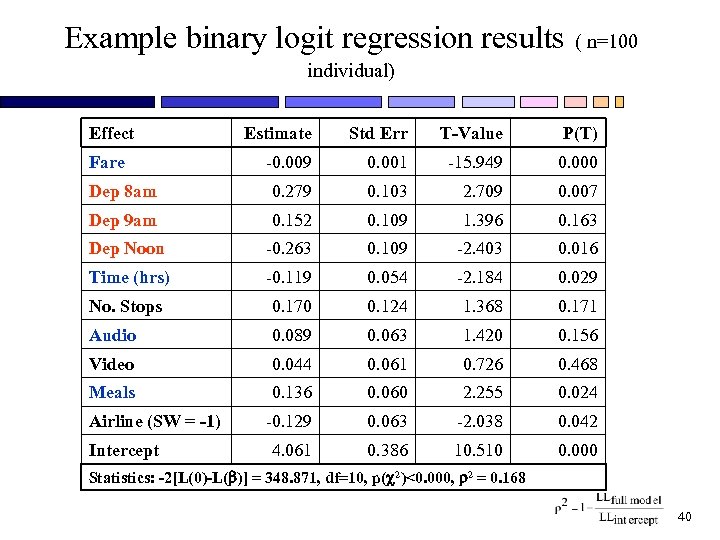Example binary logit regression results ( n=100 individual) Effect Estimate Std Err T-Value P(T) -0. 009 0. 001 -15. 949 0. 000 Dep 8 am 0. 279 0. 103 2. 709 0. 007 Dep 9 am 0. 152 0. 109 1. 396 0. 163 Dep Noon -0. 263 0. 109 -2. 403 0. 016 Time (hrs) -0. 119 0. 054 -2. 184 0. 029 No. Stops 0. 170 0. 124 1. 368 0. 171 Audio 0. 089 0. 063 1. 420 0. 156 Video 0. 044 0. 061 0. 726 0. 468 Meals 0. 136 0. 060 2. 255 0. 024 -0. 129 0. 063 -2. 038 0. 042 4. 061 0. 386 10. 510 0. 000 Fare Airline (SW = -1) Intercept Statistics: -2[L(0)-L( )] = 348. 871, df=10, p( 2)<0. 000, 2 = 0. 168 40

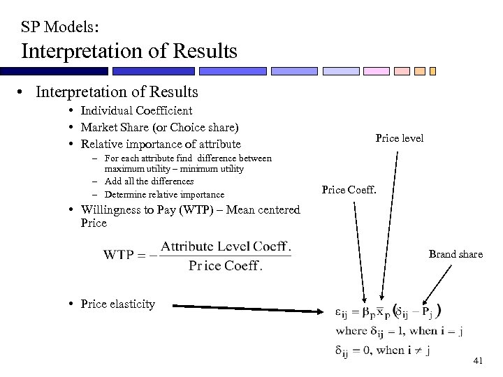SP Models: Interpretation of Results • Individual Coefficient • Market Share (or Choice share) • Relative importance of attribute – For each attribute find difference between maximum utility – minimum utility – Add all the differences – Determine relative importance Price level Price Coeff. • Willingness to Pay (WTP) – Mean centered Price Brand share • Price elasticity 41

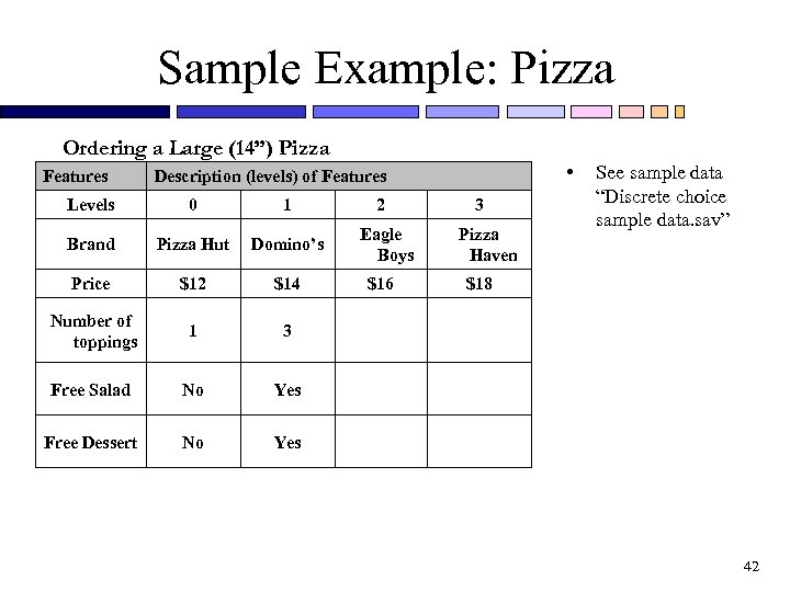Sample Example: Pizza Ordering a Large (14”) Pizza Features • Description (levels) of Features Levels 0 1 Brand Pizza Hut Domino’s Price $12 $14 Number of toppings 1 3 Free Salad No Yes Free Dessert No 2 Yes Eagle Boys $16 3 See sample data “Discrete choice sample data. sav” Pizza Haven $18 42

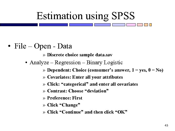Estimation using SPSS • File – Open - Data » Discrete choice sample data. sav • Analyze – Regression – Binary Logistic » » » » Dependent: Choice (consumer’s answer, 1 = yes, 0 = No) Covariates: Enter all your attributes Click: “categorical” and enter all covariates Contrast: Choose “deviation” Preference: First Click “Change” Click “Continue” and then click “OK” 43

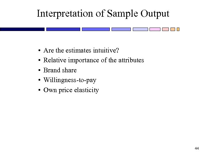Interpretation of Sample Output • • • Are the estimates intuitive? Relative importance of the attributes Brand share Willingness-to-pay Own price elasticity 44