CONDENSATION GROWTH OF CLOUD DROPLETS Growth Equation

CONDENSATION GROWTH OF CLOUD DROPLETS • Growth Equation • Examples GROWTH EQUATION When a cloud droplet grows by condensation, water vapour diffuses towards it, driven by the vapour density gradient between the environment and the surface of the drop. This vapour diffusion is governed by Fick’s Law which, assuming spherical symmetry, may be stated: (25. 1) where is the vapour mass flux (kg m-2 s-1 ), is the vapour density (kg m-3), D is the diffusion coefficient of water vapour in air (m 2 s-1), and is a unit vector pointing radially outward. Note that d /dr is positive, since the vapour diffuses down the vapour density gradient (that is, from high vapour density in the environment towards low vapour density over the surface of the drop). Mass conservation requires that: (25. 2)

where is the mass growth rate of the cloud droplet and is a spherical surface containing the droplet. Again assuming spherical symmetry of the vapour density field, Eq. 25. 2 can be combined with Eq. 25. 1 to give: (25. 3) Thus, in order to solve for the growth rate of the droplet, we need to know the vapour density gradient at some radial distance from the centre of the drop. Any distance will do, so let’s determine d /dr at the surface of the drop. If the environmental vapour field is steady (time invariant), then the continuity equation for the vapour is: (25. 4) Substituting from Eq. 25. 1 leads to a Laplace equation for the vapour density: (25. 5) which can be written in spherical coordinates (with spherical symmetry) as: (25. 6)

The general solution to Eq. 25. 6 is: (25. 7) where a, b are constants to be determined by applying the boundary conditions, namely (rd)= d, and. This leads to the specific solution: (25. 8) and finally to the vapour density gradient at the surface of the drop: (25. 9) Substituting Eq. 25. 9 into Eq. 25. 3 gives an expression for the growth rate of the drop: (25. 10) Note: One could have obtained Eq. 25. 10 more directly by simply integrating Eq. 25. 3: which leads immediately to Eq. 25. 10. We used the lengthier derivation in order to pursue the electrostatic analogy.

ASIDE ON THE ELECTROSTATIC ANALOGY Eq. 25. 10 could be obtained somewhat more simply by using an analogy with electrostatics. For droplets, this is simply an alternative way of looking at the problem. For the growth of snow crystals, however, it becomes the only way to deduce the growth equation. Let’s consider the analogy for droplets. So imagine a charge q on a spherical conductor of radius rd and capacitance C. The electrostatic analog of Eq. 25. 1 is: and Gauss’s theorem implies that: where 0 is the dielectric constant of the environment of the charged sphere. This is the analog of the mass conservation Eq. 25. 2. Substitution of gives

which is the analog of Eq. 25. 3. We also know that outside the conductor, the electric potential function (voltage) satisfies Laplace’s equation: Finally, the electrostatic problem may be formulated as follows. Given the charge on the conductor, what is the potential difference between the conductor and ground (infinity)? As you may recall from electrostatics, the ratio of the charge to the potential difference is the capacitance of the conductor, C, viz: The capacitance can be determined theoretically by following a procedure similar to the one we followed in deriving the droplet growth equation. This leads to: Which is the analog of Eq. 25. 10. The significance of this result is not so much that theory is similar for the droplet and the charged sphere, but rather that it is possible to measure the capacitance experimentally. This is especially helpful for complicated shapes such as snowflakes, where a theoretical analytical solution might not be possible, and numerical methods could be required to solve Laplace’s equation.

The condensation of vapour on the drop releases latent heat, so that a growing drop is warmer than its environment. The resulting temperature gradient allows the latent heat to be conducted away, so that the drop does not warm up indefinitely. The problem for heat conduction is analogous to that for vapour diffusion except that the sign changes (since vapour diffuses towards the drop, while heat is conducted away from it). For heat conduction, we have Fourier’s law instead of Fick’s law: (25. 11) where k is thermal conductivity of air (Wm-1 K-1 ). The outward heat flow across a spherical surface surrounding the drop must equal the rate of release of latent heat by the drop, . Hence: (25. 12) Substituting Eq. 25. 11 into Eq. 25. 12, and assuming spherical symmetry of the heat flux, leads to: (25. 13) which may be integrated, applying the boundary conditions, to give: (25. 14)

where Td , T are respectively the temperature of the droplet (strictly of its surface although we will assume it to be isothermal; please do not confuse the droplet temperature with the dewpoint temperature!) and the far-field temperature of the environment. The two equations we need to solve for the droplet growth are Eq. 25. 10 and Eq. 25. 14. However, they are incomplete, inasmuch as we may control (or measure) the environmental temperature and vapour density, but we do not know the surface temperature and vapour density of the drop. So, to complete our equations, we need two more conditions or assumptions. The first is that the system is steady. Hence the latent heat released by condensation must equal the heat conducted away from the drop. This requirement can be stated as follows: (25. 15) Substituting from Eqs. 25. 10 and 25. 14 yields: (25. 16) In order to solve Eq. 25. 16, we need to make a second assumption, known as Maxwell’s assumption, namely that the vapour density at the surface of the drop is the equilibrium vapour density over a solution drop of radius rd at temperature Td, that is d= 's, (or equivalently in terms of vapour pressure, ed=e's). Strictly speaking, this cannot be true or the drop would be in equilibrium and hence not grow. But we will assume that it will nonetheless give us a good Approximation to the vapour density at the surface of the drop.

We will begin by recasting Eq. 25. 16 in terms of vapour pressure, using the ideal gas law, and then invoking Maxwell’s assumption: (25. 17) Eq. 25. 17 can be rewritten as: (25. 18) where S is the saturation ratio in the distant environment of the drop. Note: keep in mind the different ways in which the infinity symbol is used in es( , T ). The first indicates that this is the equilibrium vapour pressure over a flat surface (inifinite radius of curvature). The infinity subscript means that this is the temperature in the distant environment of the drop. The second term in parenthesis in Eq. 25. 18 can be written: (25. 19) The first term on the RHS of Eq. 25. 19 is the Köhler curve function (rd, Td) (see Eq. 23. 6). The second term can be obtained by integrating the Clausius-Clapeyron equation from T to Td (assuming that Td-T is not too large), as follows:

(25. 20) Taking exponentials and again assuming that Td-T is small, we have finally: (25. 21) substituting from Eq. 25. 21 and Eq. 23. 6 into Eq. 25. 18 leads to an equation that can be solved for Td-T : (25. 22) where we have simplified the notation somewhat, in particular by dropping the subscript “infinity” to denote the distant environmental temperature, and dropping the “infinity” for the radius of curvature of a flat surface. Finally, we can solve for , using Eqs. 25. 14 and 25. 15 and subsituting from Eq. 25. 22. For activated solution droplets, 1, and hence:

(25. 23) Hence the mass growth rate varies linearly with droplet radius, or, equivalently, “bigger drops grow faster in mass. ” Since , we can now solve for the radial growth rate of cloud drops: (25. 24) Eq. 25. 24 can be written more simply as: (25. 25) We can think of Fk and Fd as diffusional resistances (to heat and vapour transfer, respectively) in series. They are not strong functions of temperature and pressure over the meteorological range, and so can be taken to be approximately constant. Consequently, in an environment with constant saturation ratio, Eq. 25 can be written: (25. 26)

So it appears that as a cloud drop grows by diffusion, its radial growth rate diminishes with time. Alternatively, we could say that “big drops grow more slowly in radius. ” Eq. 25. 26 can be readily integrated to give: (25. 27) where r 0 is the initial droplet radius. Thus the growth curve is parabolic, which means that as a spectrum of cloud drops grow by diffusion, the smaller ones “catch up” with the larger ones, leading to a narrowing of the size spectrum. Table 25. 1 gives an example of the growth of two drops that condense on different Na. Cl nuclei. Droplet radius ( m) Time (s) CCN mass 10 -14 g 10 -12 g 1 2. 4 0. 013 2 130 0. 61 5 1000 62 10 2700 870 20 8500 5900 30 17500 14500 50 44500 41500 Table 25. 1: Growth of two cloud droplets, T=273 K, p=90 k. Pa, S-1=0. 05% (after Mason).

Notice that the initial growth in both cases is very rapid, but that to produce typical cloud droplets of radius ten micrometres requires several tens of minutes. As an exercise, you might calculate how long it would take to produce a raindrop (r=1 mm) by condensation alone. It will convince you that rain must be produced by some other mechanism than condensational growth. Eq. 25. 27 also governs the evaporation of droplets, when c<0. If we also know the fallspeed of droplets as a function of their size, we can infer the distance required for a droplet to completely evaporate. Table 25. 2 gives some typical values. Initial droplet radius ( m) Distance fallen to evaporate 1 2 m 3 0. 17 mm 10 2. 1 cm 30 1. 7 m 100 210 m 150 1. 1 km Table 25. 2: Distance required for water droplets to evaporate. T=280 K, S=80% (Mason) The conventional boundary between cloud droplets and raindrops is a radius of 100 m. Table 25. 2 shows that raindrops are simply those drops that are large enough to reach the ground

before evaporating. Note also that drizzle has a radius of < 250 m

GROWTH OF CLOUD DROPLET POPULATIONS • A simple condensation model • Continuous growth by collision and coalescence • Stochastic collision and coalescence A SIMPLE CONDENSATION MODEL The growth of cloud droplets to a radius of about 20 m must be largely by condensation, since smaller droplets scarcely collide with other cloud droplets. We will treat the growth of a population of cloud droplets by dividing the population into a finite number of size categories and examining the growth of a “typical” droplet in each category by using the condensation growth equation. We can specify thermal conductivity, k, and the diffusivity of water vapour in air, D, as functions of T, p. Hence, we need to know something about d. T/dt, dp/dt, and d. S/dt. The saturated adiabatic lapse rate is given by (cf. 19. 7): (26. 1)

In order to determine d. S/dt, we will imagine that the saturated adiabatic process consists of a “dry” adiabatic expansion followed by an isobaric condensation. For the dry adiabatic expansion, we have: (26. 2) Setting e pr/ and assuming r=const, since there is no condensation, the first term becomes (using the hydrostatic equation and the definition of r): (26. 3) Using the Clausius-Clapeyron equation and the dry adiabatic lapse rate, the second term becomes: (26. 4) with the result that: (26. 5)

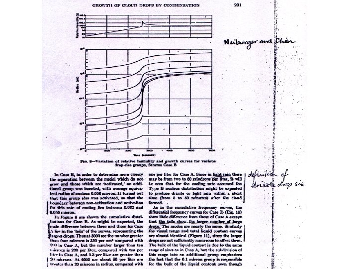
For the isobaric condensation, we have the following. Let the condensation rate by d /dt (kg of liquid water per kg of air per second). Then Eq. 26. 2 still applies, but this time the first term is: (26. 6) and the second term is: (26. 7) Finally, combining the dry adiabatic expansion and the isobaric condensation, we have: (26. 8) An example of such a growth calculation is that of Neiburger and Chien (Fig. 8). The problem is that the predicted cloud droplet spectra become narrower with time, but this is not consistent with observations. The supersaturation generally reaches its maximum (less than 0. 5%) within about 100 m of the cloud base. Note that after the initial activation, the supersaturation remains approximately constant. Then,

ignoring the solute and sphericity terms, each drop grows according to: (26. 10) But the number of drops in the size range r to r+dr must equal the number of drops in the initial size range r 0 to r 0 +dr 0. Hence n(r)dr=n(r 0)dr 0 This implies that n(r) is an increasing function of time and hence that the spectrum is narrowing, a result inconsistent with observations. Various scientists have offered different explanations for this discrepancy, including time-dependent effects in the diffusion growth equation (Borovikov), ventilation effects (due to convective heat and mass transfer), kinetic effects (Fukuta and Walter; these take into account the fact that the heat and mass transfer become discontinuous near the surface of the aroplet, due to the finite mean free path of the molecules), stochastic effects due to turbulence, and electrical effects. However, none of these effects seems to explain the magnitude of the discrepancy. One scientist (Fitzgerald) even suggested that the observations must be wrong. However, Mason suggested that the explanation of the observed broad droplet spectrum is that new embryo droplets are constantly being introduced into the cloud as a result of the horizontal entrainment of environmental air.

CONTINUOUS GROWTH BY COLLISION AND COALESCENCE Collisions between droplets occur as a result of their differential response to gravitational, electrical, and aerodynamic forces. Gravity is the major factor. Large drops fall faster than smaller ones, and hence have the opportunity to catch up and collide with them. The collision efficiency, E(R, r), for two drops of radius R and r is defined as the ratio of the actual number of collisions to the number of collisions that would occur with geometrical sweepout. If all the r-drops, initially with centres located in a cylinder of radius y, eventually collide with an R-drop, then the collision efficiency is given by: (26. 11) On collision, the drops may coalesce or the smaller drop may bounce away from the larger drop. In some collisions, the impact may lead to violent oscillations of the combined drops and eventually to breakup into two or more drops. The coalescence efficiency is simply the ratio of the number of coalescences to the number of collisions. The collection efficiency is the product of the collision and coalescence efficiencies. For the collection of cloud droplets, the coalescence efficiency is usually taken to be unity. Hence the collision and collections efficiencies are identical, and the terms are sometimes used interchangeably. In order to determine the collision rate, it is important to know the fall speed of drops from cloud droplets to rain drops. In a quiescent atmosphere, most drops will be falling at their terminal velocity. This occurs when the upward aerodynamic drag force balances the downward force

force of gravity (their weight). This balance can be expressed as: (26. 12) where Cd is the drag coefficient of the drop. We can solve Eq. 26. 12 for the terminal velocity: (26. 13) Eq. 26. 13 tells us that drops fall faster at greater altitude where the air density is lower. It also suggests that if the drag coefficient is constant, the terminal velocity varies as the square root of the drop radius. This is approximately true for large drops, with a diameter bigger than about 1 mm. I say approximately true, because water drops bigger than about 1 mm in diameter are no longer spherical. The effect of the aerodynamic drag (which tries to flatten them) overcomes the effect of surface tension (which tries to keep them spherical), with the result that large raindrops are “hamburger shaped, ” and their shape varies with drop size, with the result that the drag coefficient is dependent on drop radius. The terminal velocity of smaller drops actually varies as the square of the radius. This can be seen by introducing the Reynolds number into Eq. 26. 12: (26. 14)

where a is the dynamic viscosity of air. The left hand side of Eq. 26. 12 (the drag) may then be written: (26. 15) The quantity outside the parenthesis on the right hand side of Eq. 26. 15 is called the Stokes drag. for drops with Re<<1, the quantity in parenthesis is unity, hence for small drops (cloud drops) the drag is proportional to radius. Solving Eq. 26. 12 again for the terminal velocity leads to: (26. 16) Thus for cloud droplets with Re<<1, the terminal velocity varies as the square of the radius. Table 26. 1 gives experimental values of the terminal velocity of water drops of various sizes falling through air:

Drop diameter ( m) Terminal velocity (cms-1) 10 0. 3 50 7. 2 100 25. 6 500 204 1000 403 5000 909 Table 26. 1: Terminal velocity of water drops at a pressure of 1 atmosphere and a temperature of 20 o C. Note: the large drop diameters are the equivalent spherical diameter of these large “hamburger shaped” drops. That is, the diameter of a spherical drop with the same mass. Raindrops much larger than this generally tend to be aerodynamically unstable and break up spontaneously. Note the r 2 dependence of the terminal velocity for the first two drop sizes in Table 26. 1 and the r 0. 5 dependence for the last two categories. The two intermediate size drops (drizzle drops) have an approximately linear dependence of terminal velocity on radius (or diameter). We now have the necessary tools to derive an equation for the growth rate of large drops. We begin by making the continuum assumption (hence continuous growth). What this means is that we will ignore the specifics of individual collisions. We will even ignore the fact that the smaller drops which it collects are individual drops. Rather, we will imagine that the cloud water is distributed continuously in space with a liquid water content M (kg m-3 ). We will even assume, for now, that the big drop collects all of the cloud water in its geometrically swept-out

path. Thus in unit time, the big drop (radius R) sweeps out a volume of R 2 v(R). Therefore, the water mass collected by the big drop in unit time is R 2 v(R)M and this must equal the mass growth rate of the drop, which is l 4 R 2 d. R/dt. Hence, solving for the radial growth rate: (26. 17) At this point we will acknowledge that in reality the drop will not sweep out all of this water, because some of the smaller drops will flow around the big drop in the airstream (and some may bounce and not coalesce). In order to allow for this, we will introduce an average collection efficiency on the right hand side of Eq. 26. 17: (26. 18) Eq. 26. 18 is the classical continuous growth equation.