Computer Vision Affine structure from motion Marc Pollefeys

Computer Vision Affine structure from motion Marc Pollefeys COMP 256 Some slides and illustrations from J. Ponce, A. Zisserman, R. Hartley, Luc Van Gool, …

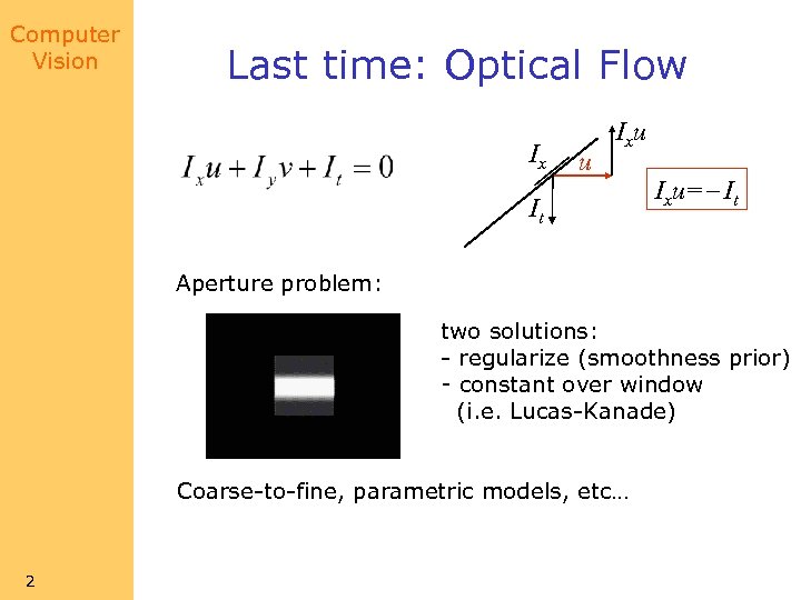Computer Vision Last time: Optical Flow Ix u It Ixu=- It Aperture problem: two solutions: - regularize (smoothness prior) - constant over window (i. e. Lucas-Kanade) Coarse-to-fine, parametric models, etc… 2

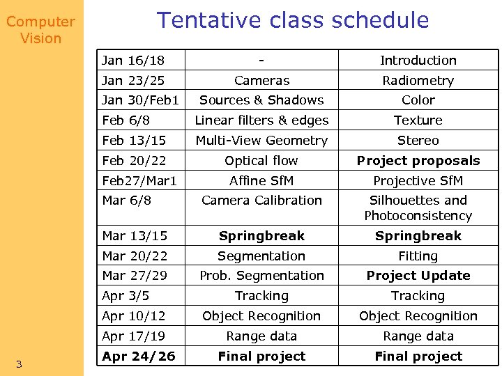Tentative class schedule Computer Vision Jan 16/18 - Introduction Jan 23/25 Cameras Radiometry Sources & Shadows Color Feb 6/8 Linear filters & edges Texture Feb 13/15 Multi-View Geometry Stereo Feb 20/22 Optical flow Project proposals Affine Sf. M Projective Sf. M Camera Calibration Silhouettes and Photoconsistency Mar 13/15 Springbreak Mar 20/22 Segmentation Fitting Mar 27/29 Prob. Segmentation Project Update Tracking Apr 10/12 Object Recognition Apr 17/19 Range data Final project Jan 30/Feb 1 Feb 27/Mar 1 Mar 6/8 Apr 3/5 3 Apr 24/26

Computer Vision AFFINE STRUCTURE FROM MOTION • The Affine Structure from Motion Problem • Elements of Affine Geometry • Affine Structure from Motion from two Views • A Geometric Approach • Affine Epipolar Geometry • An Algebraic Approach • Affine Structure from Motion from Multiple Views • From Affine to Euclidean Images • Structure from motion of multiple and deforming object Reading: Chapter 12. 4

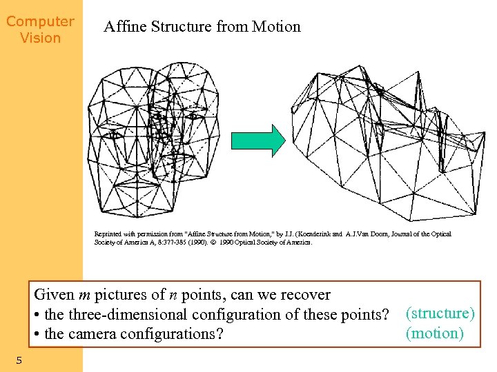Computer Vision Affine Structure from Motion Reprinted with permission from “Affine Structure from Motion, ” by J. J. (Koenderink and A. J. Van Doorn, Journal of the Optical Society of America A, 8: 377 -385 (1990). 1990 Optical Society of America. Given m pictures of n points, can we recover • the three-dimensional configuration of these points? • the camera configurations? 5 (structure) (motion)

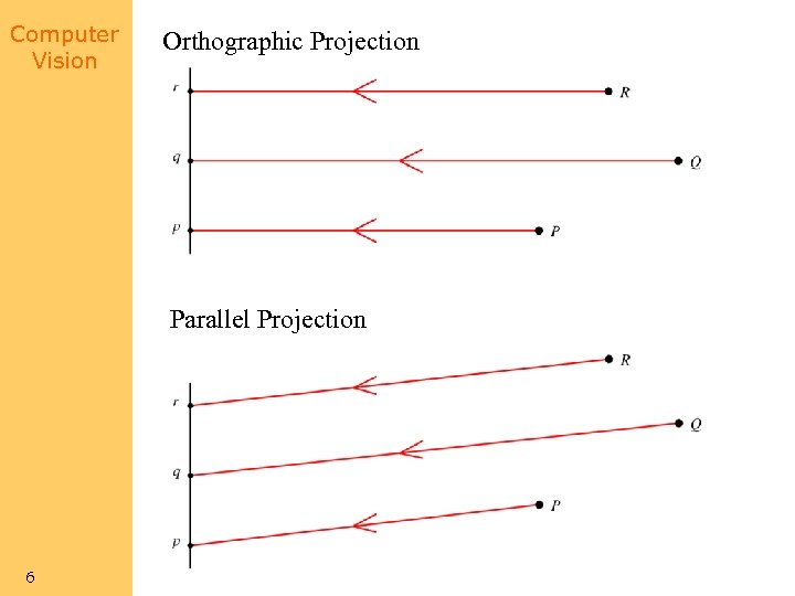Computer Vision Orthographic Projection Parallel Projection 6

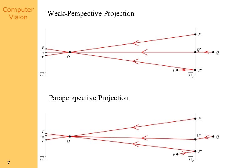Computer Vision Weak-Perspective Projection Paraperspective Projection 7

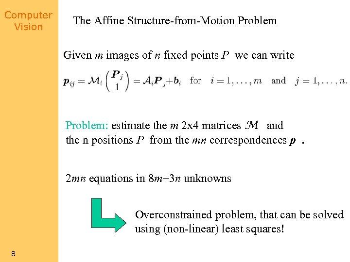Computer Vision The Affine Structure-from-Motion Problem Given m images of n fixedj points P we can write Problem: estimate the m 2 x 4 matrices M i and the n positions P j from the mn correspondences p. ij 2 mn equations in 8 m+3 n unknowns Overconstrained problem, that can be solved using (non-linear) least squares! 8

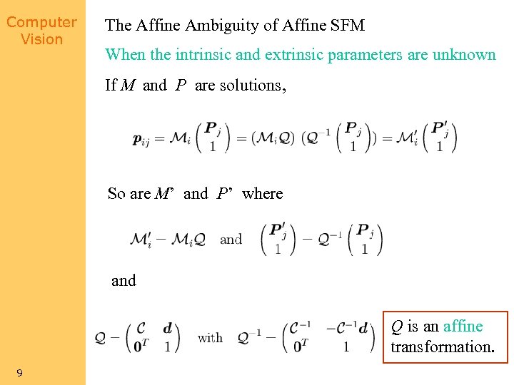Computer Vision The Affine Ambiguity of Affine SFM When the intrinsic and extrinsic parameters are unknown If M i and P are solutions, j So are M’ and P’ where i j and Q is an affine transformation. 9

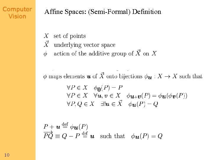Computer Vision 10 Affine Spaces: (Semi-Formal) Definition

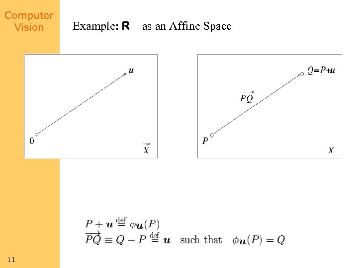Computer Vision 11 2 Example: R as an Affine Space

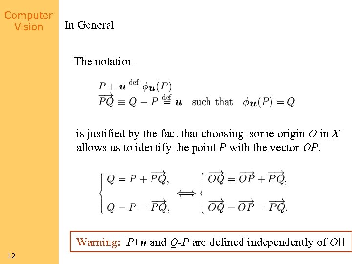Computer Vision In General The notation is justified by the fact that choosing some origin O in X allows us to identify the point P with the vector OP. Warning: P+u and Q-P are defined independently of O!! 12

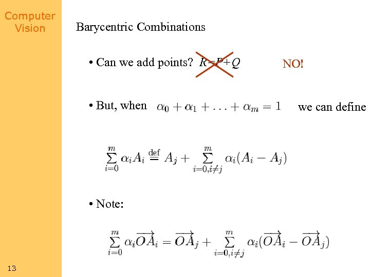Computer Vision Barycentric Combinations • Can we add points? R=P+Q • But, when • Note: 13 NO! we can define

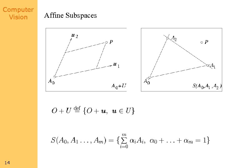Computer Vision 14 Affine Subspaces

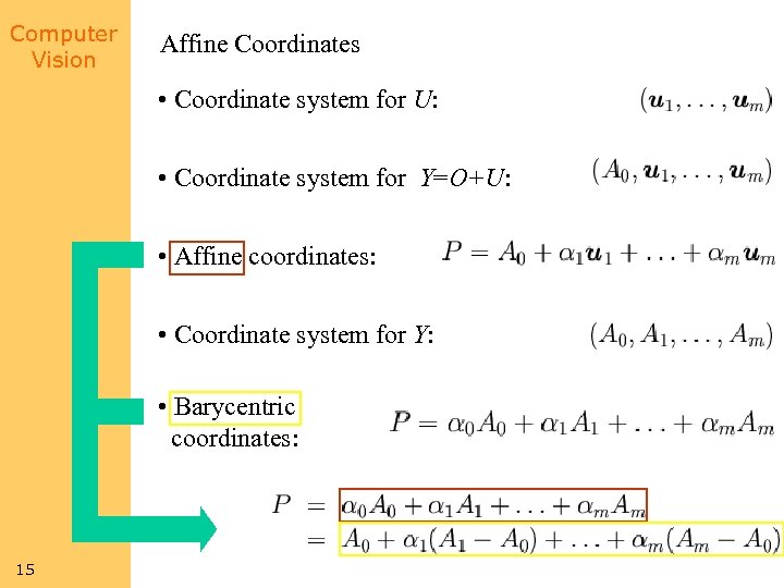Computer Vision Affine Coordinates • Coordinate system for U: • Coordinate system for Y=O+U: • Affine coordinates: • Coordinate system for Y: • Barycentric coordinates: 15

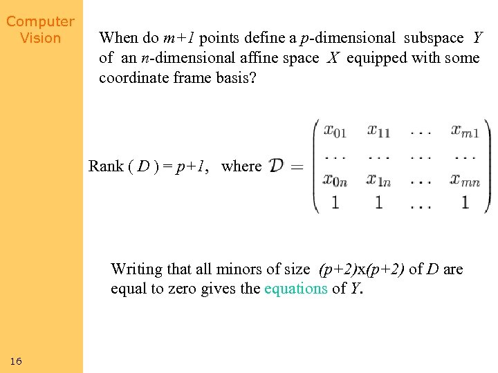Computer Vision When do m+1 points define a p-dimensional subspace Y of an n-dimensional affine space X equipped with some coordinate frame basis? Rank ( D ) = p+1, where Writing that all minors of size (p+2)x(p+2) of D are equal to zero gives the equations of Y. 16

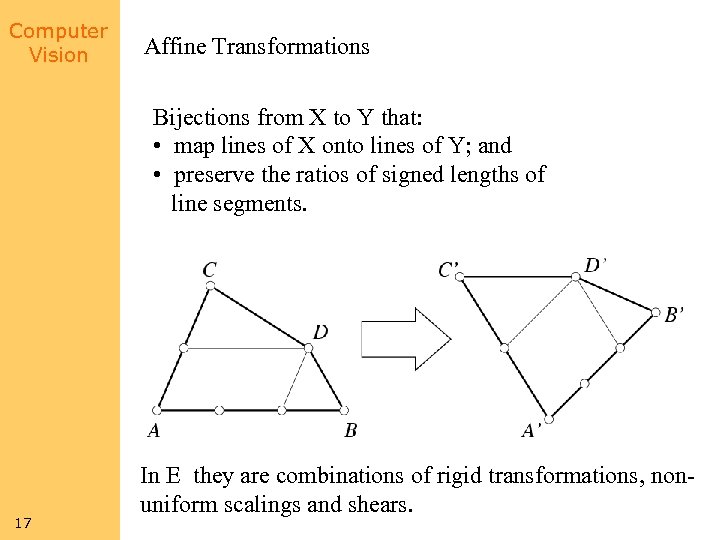Computer Vision Affine Transformations Bijections from X to Y that: • Bijections from X to Y that: map m-dimensional subspaces of X onto m-dimensional • subspaces of Y; onto lines of Y; and map lines of X preserve the ratios of onto parallel of • • map parallel subspacessigned lengthssubspaces; and line segments. • preserve affine (or barycentric) coordinates. 17 3 In E they are combinations of rigid transformations, nonuniform scalings and shears.

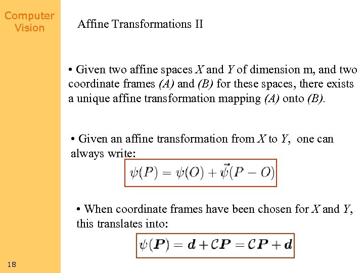Computer Vision Affine Transformations II • Given two affine spaces X and Y of dimension m, and two coordinate frames (A) and (B) for these spaces, there exists a unique affine transformation mapping (A) onto (B). • Given an affine transformation from X to Y, one can always write: • When coordinate frames have been chosen for X and Y, this translates into: 18

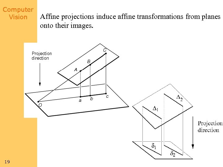Computer Vision 19 Affine projections induce affine transformations from planes onto their images.

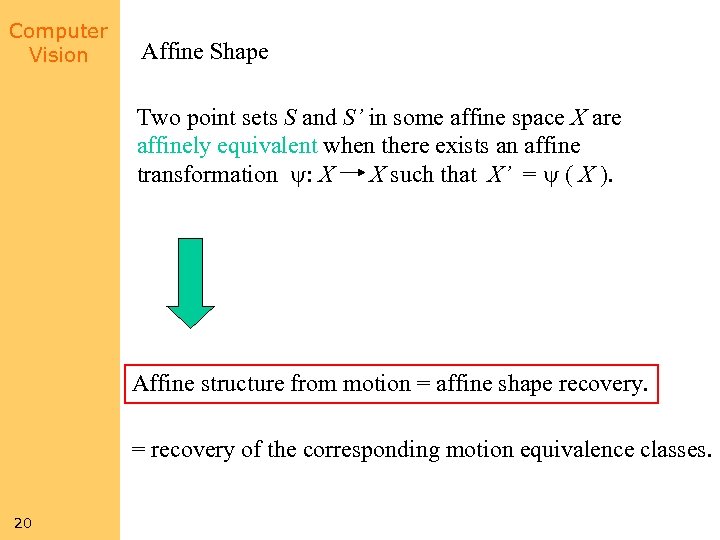Computer Vision Affine Shape Two point sets S and S’ in some affine space X are affinely equivalent when there exists an affine transformation y: X X such that X’ = y ( X ). Affine structure from motion = affine shape recovery. = recovery of the corresponding motion equivalence classes. 20

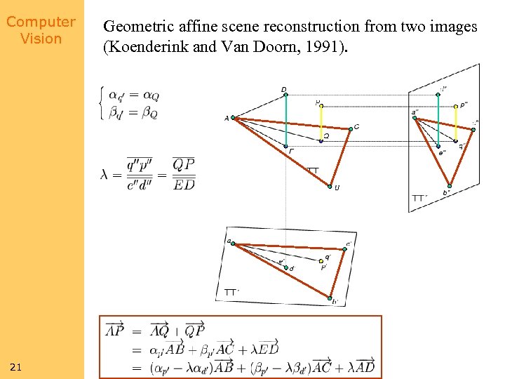Computer Vision 21 Geometric affine scene reconstruction from two images (Koenderink and Van Doorn, 1991).

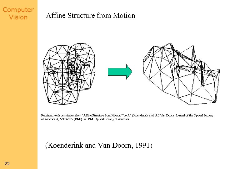Computer Vision Affine Structure from Motion Reprinted with permission from “Affine Structure from Motion, ” by J. J. (Koenderink and A. J. Van Doorn, Journal of the Optical Society of America A, 8: 377 -385 (1990). 1990 Optical Society of America. (Koenderink and Van Doorn, 1991) 22

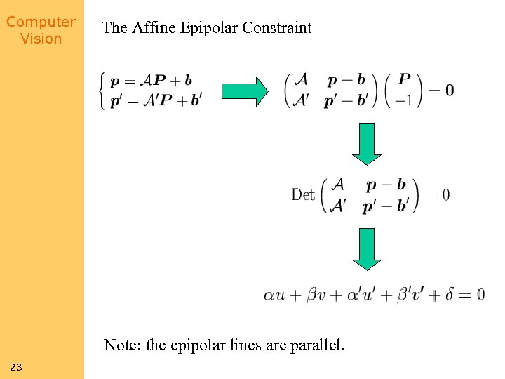Computer Vision The Affine Epipolar Constraint Note: the epipolar lines are parallel. 23

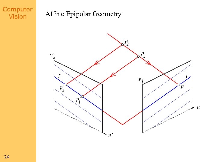Computer Vision 24 Affine Epipolar Geometry

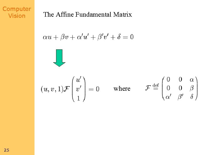Computer Vision The Affine Fundamental Matrix where 25

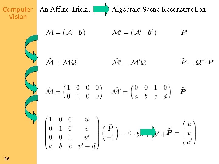Computer Vision 26 An Affine Trick. . Algebraic Scene Reconstruction

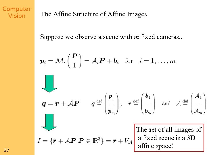Computer Vision The Affine Structure of Affine Images Suppose we observe a scene with m fixed cameras. . 27 The set of all images of a fixed scene is a 3 D affine space!

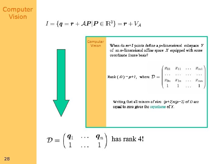Computer Vision has rank 4! 28

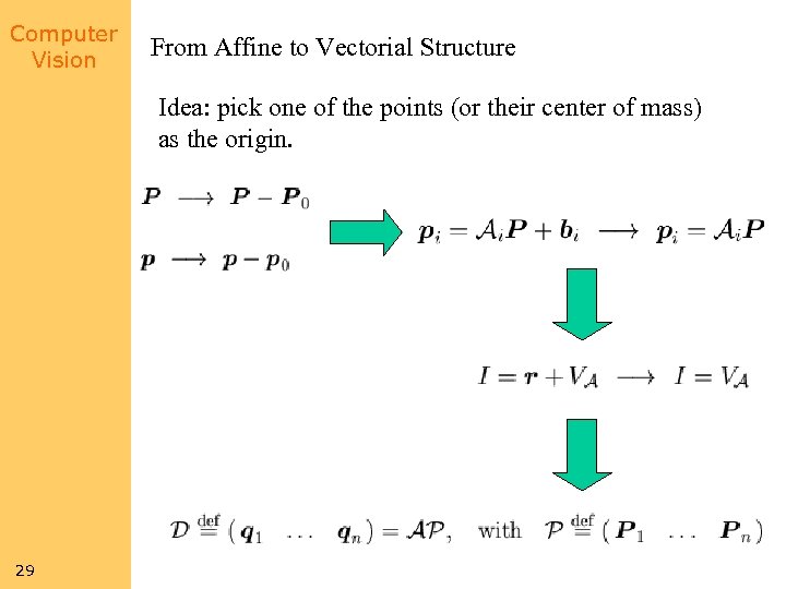Computer Vision From Affine to Vectorial Structure Idea: pick one of the points (or their center of mass) as the origin. 29

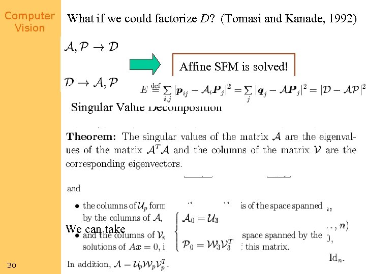Computer Vision What if we could factorize D? (Tomasi and Kanade, 1992) Affine SFM is solved! Singular Value Decomposition We can take 30

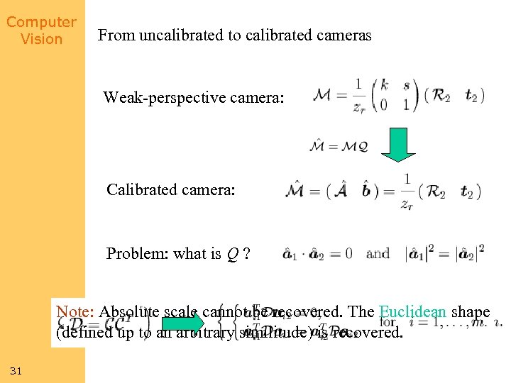Computer Vision From uncalibrated to calibrated cameras Weak-perspective camera: Calibrated camera: Problem: what is Q ? Note: Absolute scale cannot be recovered. The Euclidean shape (defined up to an arbitrary similitude) is recovered. 31

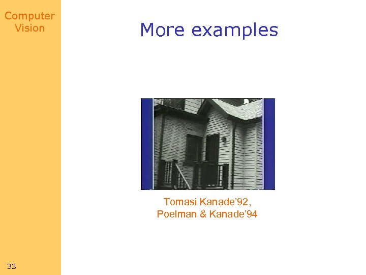
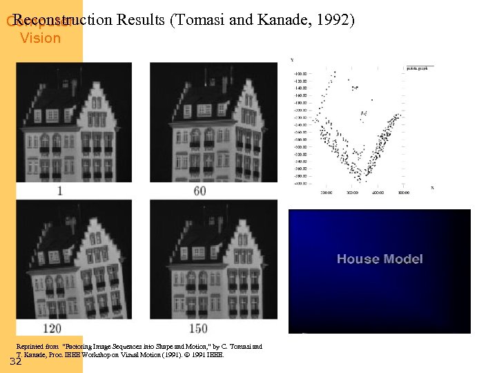Reconstruction Computer Vision Results (Tomasi and Kanade, 1992) Reprinted from “Factoring Image Sequences into Shape and Motion, ” by C. Tomasi and T. Kanade, Proc. IEEE Workshop on Visual Motion (1991). 1991 IEEE. 32

Computer Vision More examples Tomasi Kanade’ 92, Poelman & Kanade’ 94 33

Computer Vision More examples Tomasi Kanade’ 92, Poelman & Kanade’ 94 34

Computer Vision More examples Tomasi Kanade’ 92, Poelman & Kanade’ 94 35

Computer Vision Further Factorization work Factorization with uncertainty (Irani & Anandan, IJCV’ 02) Factorization for indep. moving objects (now) (Costeira and Kanade ‘ 94) Factorization for articulated objects (now) (Yan and Pollefeys ‘ 05) Factorization for dynamic objects (now) (Bregler et al. 2000, Brand 2001) Perspective factorization (next week) (Sturm & Triggs 1996, …) Factorization with outliers and missing pts. 36 (Jacobs ‘ 97 (affine), Martinek & Pajdla‘ 01 Aanaes’ 02 (perspective))

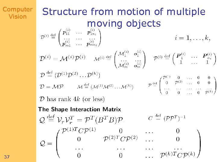Computer Vision 37 Structure from motion of multiple moving objects

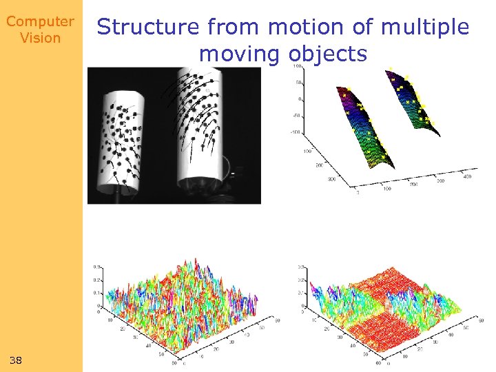Computer Vision 38 Structure from motion of multiple moving objects

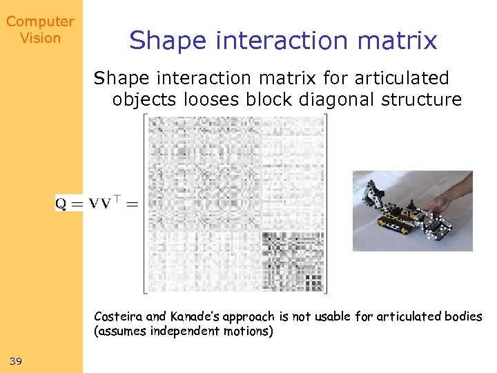Computer Vision Shape interaction matrix for articulated objects looses block diagonal structure Costeira and Kanade’s approach is not usable for articulated bodies (assumes independent motions) 39

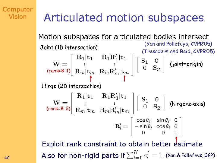Computer Vision Articulated motion subspaces Motion subspaces for articulated bodies intersect Joint (1 D intersection) (rank=8 -1) (Yan and Pollefeys, CVPR’ 05) (Tresadern and Reid, CVPR’ 05) (joint=origin) Hinge (2 D intersection) (rank=8 -2) (hinge=z-axis) Exploit rank constraint to obtain better estimate 40 Also for non-rigid parts if (Yan & Pollefeys, 06? )

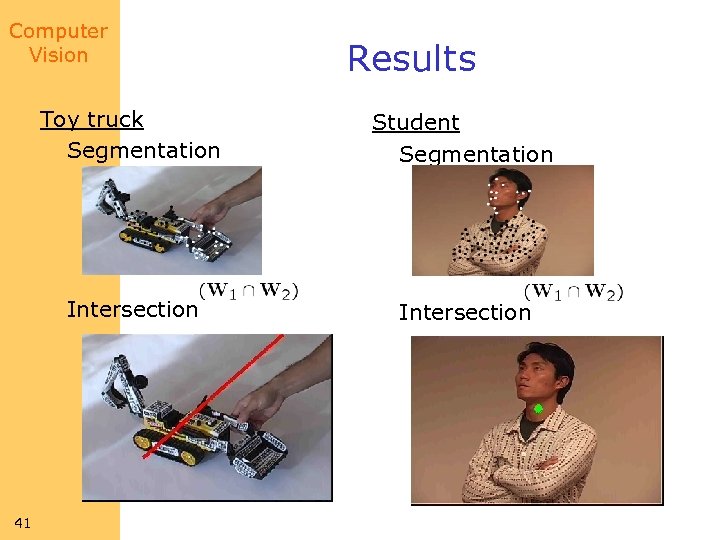Computer Vision Results Toy truck Segmentation Intersection 41 Student Segmentation Intersection

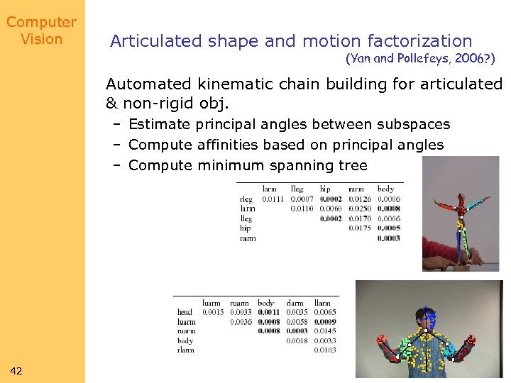Computer Vision Articulated shape and motion factorization (Yan and Pollefeys, 2006? ) Automated kinematic chain building for articulated & non-rigid obj. – Estimate principal angles between subspaces – Compute affinities based on principal angles – Compute minimum spanning tree 42

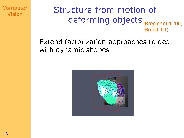Computer Vision Structure from motion of deforming objects (Bregler et al ’ 00; Brand ‘ 01) Extend factorization approaches to deal with dynamic shapes 43

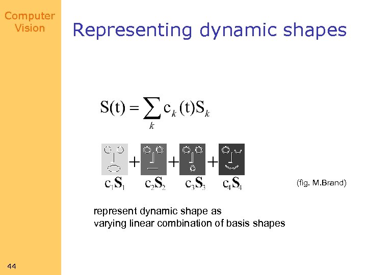Computer Vision Representing dynamic shapes (fig. M. Brand) represent dynamic shape as varying linear combination of basis shapes 44

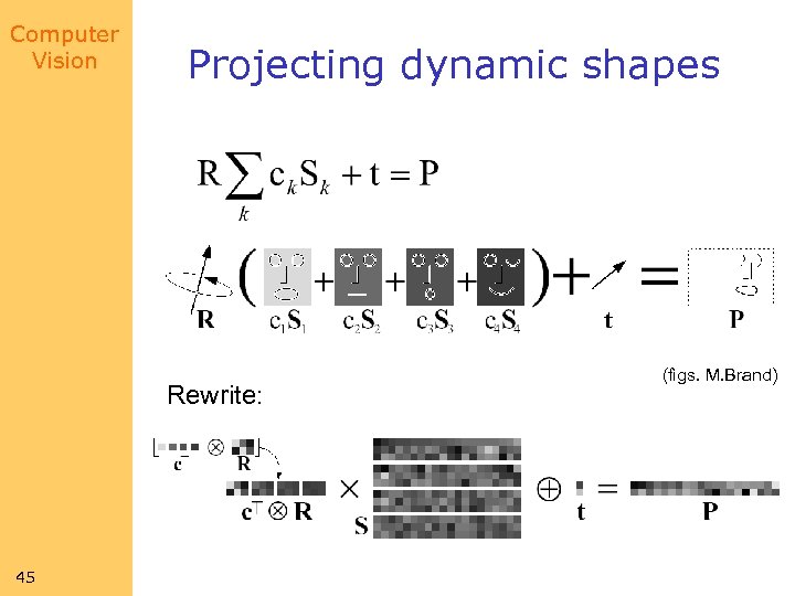Computer Vision Projecting dynamic shapes Rewrite: 45 (figs. M. Brand)

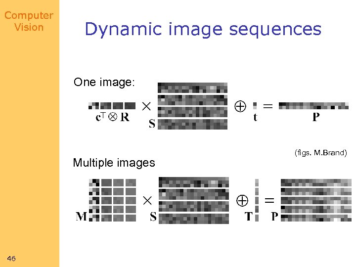Computer Vision Dynamic image sequences One image: Multiple images 46 (figs. M. Brand)

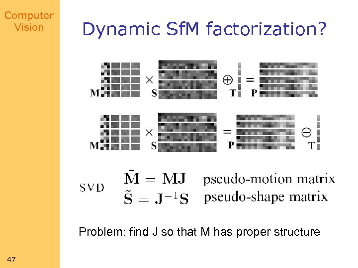Computer Vision Dynamic Sf. M factorization? Problem: find J so that M has proper structure 47

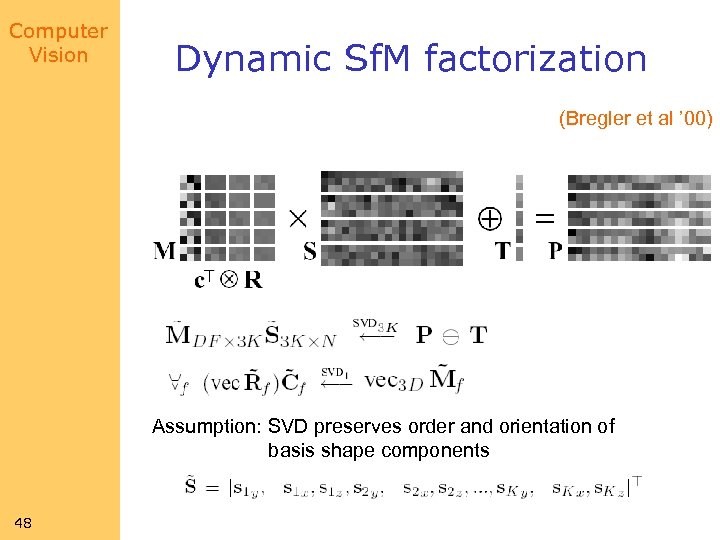Computer Vision Dynamic Sf. M factorization (Bregler et al ’ 00) Assumption: SVD preserves order and orientation of basis shape components 48

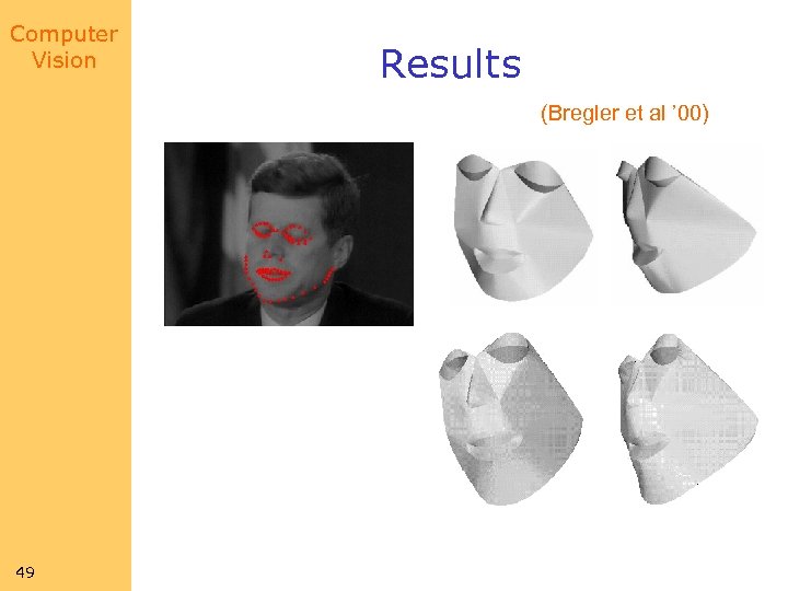Computer Vision Results (Bregler et al ’ 00) 49

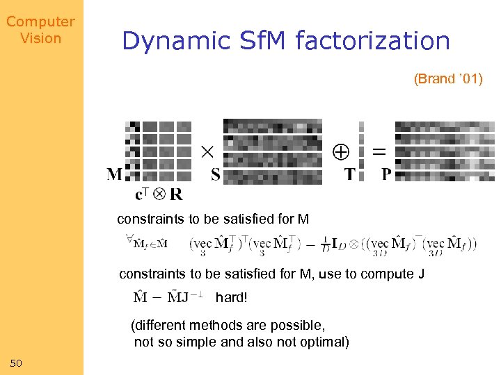Computer Vision Dynamic Sf. M factorization (Brand ’ 01) constraints to be satisfied for M, use to compute J hard! (different methods are possible, not so simple and also not optimal) 50

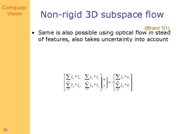Computer Vision Non-rigid 3 D subspace flow (Brand ’ 01) • Same is also possible using optical flow in stead of features, also takes uncertainty into account 51

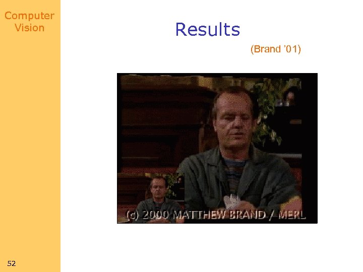Computer Vision Results (Brand ’ 01) 52

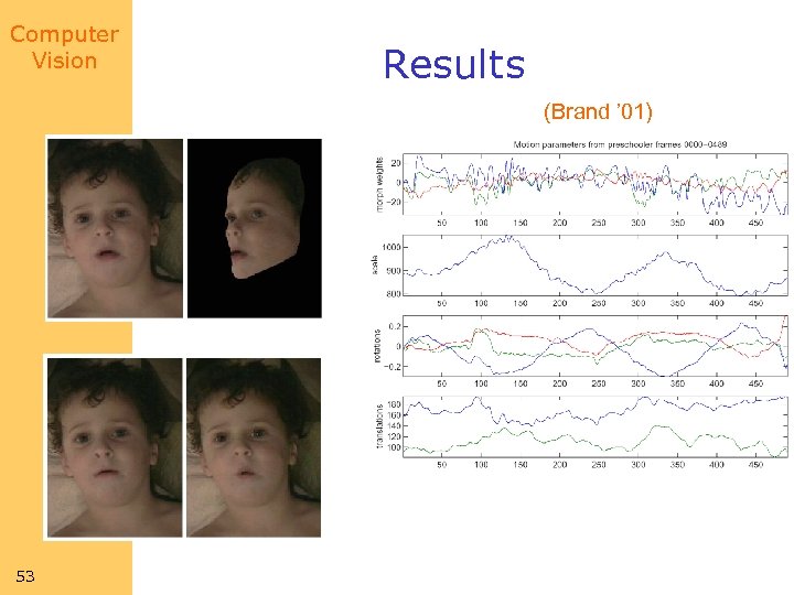Computer Vision Results (Brand ’ 01) 53

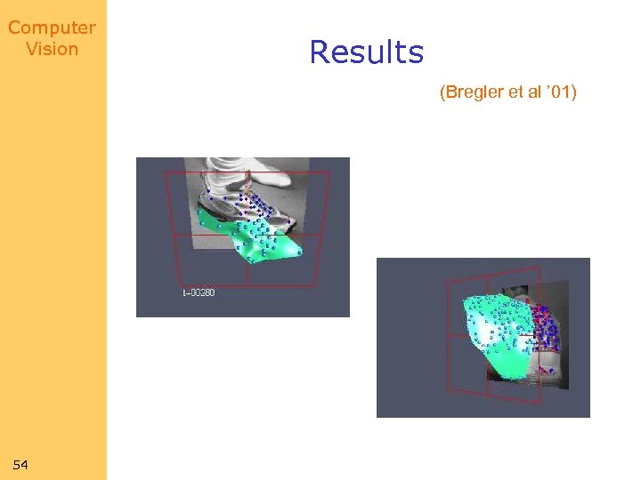Computer Vision Results (Bregler et al ’ 01) 54

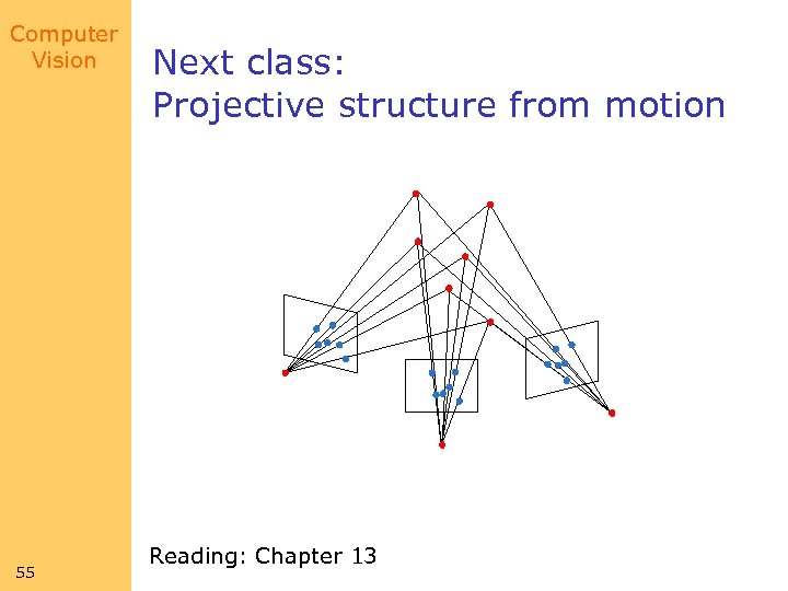Computer Vision 55 Next class: Projective structure from motion Reading: Chapter 13