Computer Modeling and Visualization in Chemistry Spring 2007

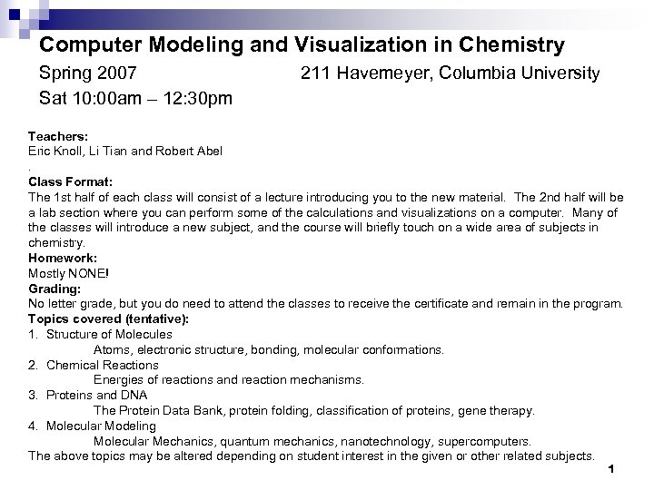Computer Modeling and Visualization in Chemistry Spring 2007 Sat 10: 00 am – 12: 30 pm 211 Havemeyer, Columbia University Teachers: Eric Knoll, Li Tian and Robert Abel. Class Format: The 1 st half of each class will consist of a lecture introducing you to the new material. The 2 nd half will be a lab section where you can perform some of the calculations and visualizations on a computer. Many of the classes will introduce a new subject, and the course will briefly touch on a wide area of subjects in chemistry. Homework: Mostly NONE! Grading: No letter grade, but you do need to attend the classes to receive the certificate and remain in the program. Topics covered (tentative): 1. Structure of Molecules Atoms, electronic structure, bonding, molecular conformations. 2. Chemical Reactions Energies of reactions and reaction mechanisms. 3. Proteins and DNA The Protein Data Bank, protein folding, classification of proteins, gene therapy. 4. Molecular Modeling Molecular Mechanics, quantum mechanics, nanotechnology, supercomputers. The above topics may be altered depending on student interest in the given or other related subjects. 1

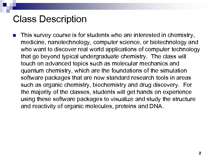Class Description n This survey course is for students who are interested in chemistry, medicine, nanotechnology, computer science, or biotechnology and who want to discover real world applications of computer technology that go beyond typical undergraduate chemistry. The class will touch on advanced topics such as molecular mechanics and quantum chemistry, which are the foundations of the simulation software packages that are now standard research tools in areas such as organic chemistry, biochemistry and drug discovery. For the majority of the classes, students will get hands on experience using these software packages to visualize and study the structure and reactivity of organic molecules, proteins and DNA. 2

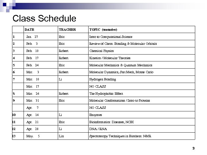Class Schedule DATE TEACHER TOPIC (tentative) 1 Jan. 27 Eric Intro to Computational Science 2 Feb. Eric Review of Chem. Bonding & Molecular Orbitals 3 Feb. 10 Robert Chemical Physics 4 Feb. 17 Robert Kinetics / Molecular Theories 5 Feb. 24 Eric Molecular Mechanics & Quantum Mechanics 6 Mar. Robert Molecular Dynamics, Stat Mech, Monte Carlo 7 Mar. 10 Li Hydrogen Bonding Mar. 17 8 Mar. 24 Robert The Hydrophobic Effect 9 Mar. 31 Eric Molecular Conformations / Intro to Proteins Apr. 10 Apr. 14 Li Enzymes 11 Apr. 21 Eric Bioinformatics: Diseases, NCBI 12 Apr. 28 Li DNA / RNA 13 May. Lin Spectroscopy Techniques in Biochem: NMR 3 3 NO CLASS 7 5 NO CLASS 3

- Science Honors Program Computer Modeling and Visualization in Chemistry Computational Science Eric Knoll 4

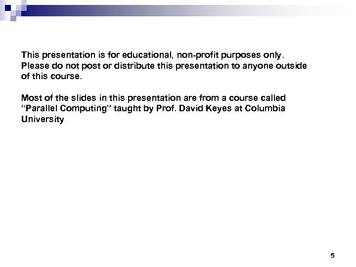This presentation is for educational, non-profit purposes only. Please do not post or distribute this presentation to anyone outside of this course. Most of the slides in this presentation are from a course called “Parallel Computing” taught by Prof. David Keyes at Columbia University 5

Three “pillars” of scientific investigation n Experiment Theory Simulation (“theoretical experiments”) Computational simulation : = “a means of scientific discovery that employs a computer system to simulate a physical system according to laws derived from theory and experiment” 6

“There will be opened a gateway and a road to a large and excellent science into which minds more piercing than mine shall penetrate to recesses still deeper. ” Galileo (1564 -1642) (on ‘experimental mathematical analysis of nature’ appropriated here for ‘simulation science’) 7

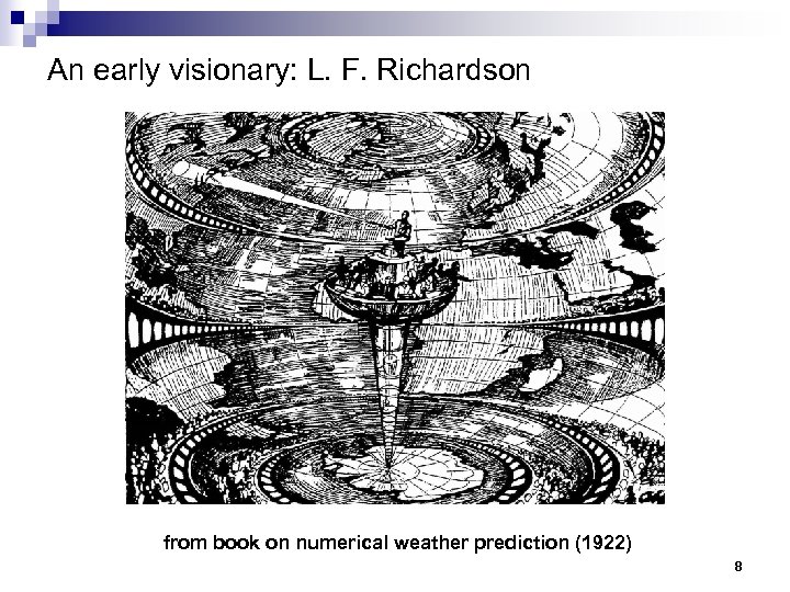An early visionary: L. F. Richardson from book on numerical weather prediction (1922) 8

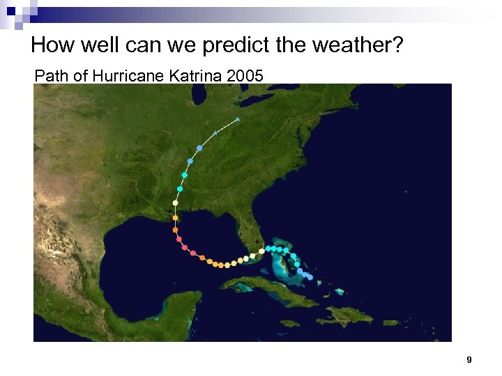How well can we predict the weather? Path of Hurricane Katrina 2005 9

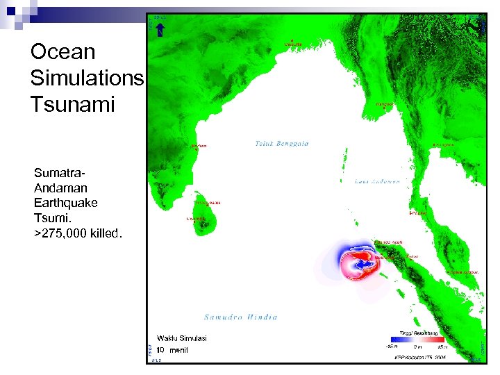Ocean Simulations Tsunami Sumatra. Andaman Earthquake Tsumi. >275, 000 killed. 10

The third pillar n n Computational science has been the stuff of fantasy for generations (Galileo, Richardson, etc. ) Modern version, hosted on digital computers, has been foreseen for about 60 years (Von Neumann, 1946) Aggressively promoted as a national agenda for about 15 years (Wilson, 1989) Just now beginning to earn acceptance beyond the circle of practitioners Experimental publication: except for the team that did the experiments, everybody believes it Computational publication: except for the team that did the computations, nobody believes it. 11

The “Grand Challenges” of Wilson n n n A Magna Carta of high performance computing (1989) Supercomputer as “scientific instrument” Attention to quality research indicators in computational science Sample “grand challenge” – electronic structure Prospects for computer technology Why the NSF supercomputer centers 12

Wilson’s burden “In this paper, I address some of the tougher requirements on … grand challenge research to ensure that is has enduring value. ” ¨ Algorithm development ¨ Error control ¨ Software productivity ¨ Fostering technological advances in computers 13

Wilson’s fear “… Often advocated is that because computers of a fixed performance are dropping rapidly in price, one should only buy inexpensive computers … expecting that today’s supercomputer performance will be achieved … in a few years’ time. This … would be terrible… It would violate the whole spirit of science, of pushing at the frontiers of knowledge and technology simultaneously. ” 14

Wilson’s six examples n n n Weather prediction Astronomy Materials science Molecular biology Aerodynamics Quantum field theory 15

Wilson’s six examples n Weather prediction ¨ curse of dimensionality (r 3 in space; r 4 in time) ¨ chaotic behavior n n n Astronomy Materials science Molecular biology Aerodynamics Quantum field theory 16

Wilson’s six examples n n Weather prediction Astronomy ¨ need to escape limits of observational record ¨ curse of dimensionality n n Materials science Molecular biology Aerodynamics Quantum field theory 17

Wilson’s six examples n n n Weather prediction Astronomy Materials science ¨ Electronic structure problem: 3 N-dimensional ¨ Schroedinger way behind Newton, Maxwell n n n Molecular biology Aerodynamics Quantum field theory 18

Wilson’s six examples n n Weather prediction Astronomy Materials science Molecular biology ¨ Conformation problem combinatorial ¨ Protein folding “stiff” n n Aerodynamics Quantum field theory 19

Wilson’s six examples n n n Weather prediction Astronomy Materials science Molecular biology Aerodynamics ¨ Turbulence ¨ Full n system analysis, full envelope analysis Quantum field theory 20

Wilson’s six examples n n n Weather prediction Astronomy Materials science Molecular biology Aerodynamics Quantum field theory ¨ QED is perturbative ¨ QCD is fundamentally nonlinear 21

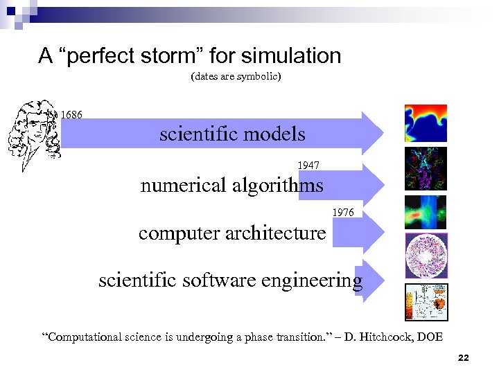A “perfect storm” for simulation (dates are symbolic) Hardware Infrastructure Applications 1686 A R C H I T E C T U R E S scientific models 1947 numerical algorithms 1976 computer architecture scientific software engineering “Computational science is undergoing a phase transition. ” – D. Hitchcock, DOE 22

Movement towards simulation science n Standards ¨ ¨ n Publications ¨ ¨ n Tools: languages, libraries, interfaces, formats, templates Results: validation and verification Journals, e. g. , IEEE/APS Computing in Science and Engineering Book series, e. g. , Springer’s LNCS&E Degree programs ¨ Approximately 50 US-based programs http: //www. nhse. org/cse_edu. html ¨ Birds-of-a-feather meetings at conferences 23

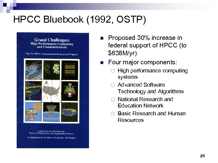HPCC Bluebook (1992, OSTP) n n Proposed 30% increase in federal support of HPCC (to $638 M/yr) Four major components: High performance computing systems ¨ Advanced Software Technology and Algorithms ¨ National Research and Education Network ¨ Basic Research and Human Resources ¨ 25

It’s not just government… n 200 of the “Top 500” computer systems in the world are operated by industry http: //www. top 500. org/ n 15 “Fortune 500” companies were sponsors of the NCSA ¨ ¨ ¨ ¨ Banking: J. P. Morgan Information: The Tribune Company Insurance: Allstate Manufacturing: Caterpillar, FMC, Kodak, Motorola Merchandising: Sears Petroleum: Phillips, Schlumberger, Shell Pharmaceuticals: Lilly Transportation: Boeing, Ford, SABRE 27

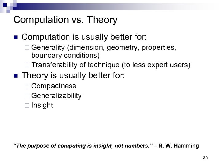Computation vs. Theory n Computation is usually better for: ¨ Generality (dimension, geometry, properties, boundary conditions) ¨ Transferability of technique (to less expert users) n Theory is usually better for: ¨ Compactness ¨ Generalizability ¨ Insight “The purpose of computing is insight, not numbers. ” – R. W. Hamming 28

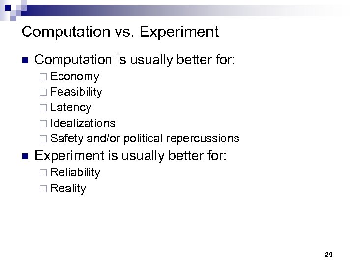Computation vs. Experiment n Computation is usually better for: ¨ Economy ¨ Feasibility ¨ Latency ¨ Idealizations ¨ Safety n and/or political repercussions Experiment is usually better for: ¨ Reliability ¨ Reality 29

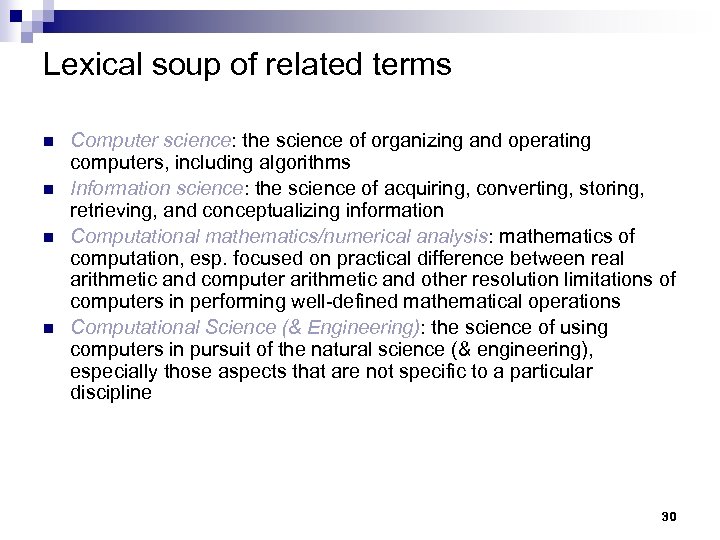Lexical soup of related terms n n Computer science: the science of organizing and operating computers, including algorithms Information science: the science of acquiring, converting, storing, retrieving, and conceptualizing information Computational mathematics/numerical analysis: mathematics of computation, esp. focused on practical difference between real arithmetic and computer arithmetic and other resolution limitations of computers in performing well-defined mathematical operations Computational Science (& Engineering): the science of using computers in pursuit of the natural science (& engineering), especially those aspects that are not specific to a particular discipline 30

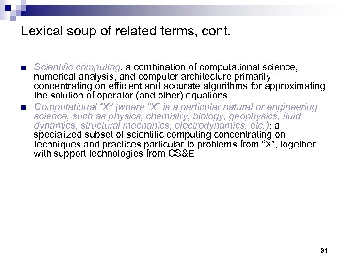Lexical soup of related terms, cont. n n Scientific computing: a combination of computational science, numerical analysis, and computer architecture primarily concentrating on efficient and accurate algorithms for approximating the solution of operator (and other) equations Computational “X” (where “X” is a particular natural or engineering science, such as physics, chemistry, biology, geophysics, fluid dynamics, structural mechanics, electrodynamics, etc. ): a specialized subset of scientific computing concentrating on techniques and practices particular to problems from “X”, together with support technologies from CS&E 31

Clarifying examples n n Computer science: architecture, systems software, data structures, algorithmic complexity, networks, software engineering, intelligent agents, profiling, benchmarking, performance modeling, performance tuning Information science: data bases, data mining, data compression, pattern recognition Computational mathematics: error analysis, algorithmic stability, convergence Computational science: scientific visualization, computational steering, parallel partitioning and mapping, multidisciplinary computing 32

Case studies from O’Leary (1997) n Cellular radio transmission --- placement of transmitters in building to avoid dead spots (50% physics/engineering, 10% numerical analysis, 40% computer science) ¨ n Image processing --- correction of Hubble images (25% astronomy, 25% signal processing, 25% mathematics, 25% computer science) ¨ n Singular value decomposition Smoke plume modeling --- predict spread of smoke and heat in burning building (25% physics/engineering, 50% mathematics, 25% computer science) ¨ n Large, ill-conditioned inverse problem Information retrieval --- latent semantic indexing of large data bases (50% disciplinary field, 10% mathematics, 40% computer science) ¨ n Ray tracing, attenuation modeling Large scale parallel, uncertainty quantification What does Computational Chemistry Involve? 33

Single Processor 34

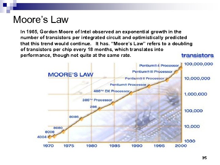Moore’s Law In 1965, Gordon Moore of Intel observed an exponential growth in the number of transistors per integrated circuit and optimistically predicted that this trend would continue. It has. “Moore’s Law” refers to a doubling of transistors per chip every 18 months, which translates into performance, though not quite at the same rate. 35

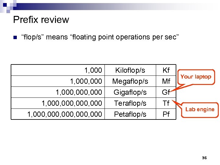Prefix review n “flop/s” means “floating point operations per sec” 1, 000, 000, 000 Kiloflop/s Megaflop/s Gigaflop/s Teraflop/s Kf Mf Gf Tf 1, 000, 000 Petaflop/s Pf Your laptop Lab engine 36

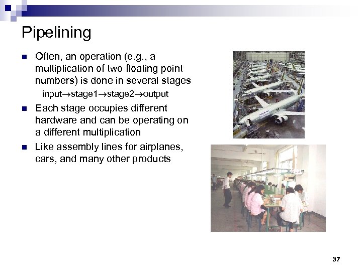Pipelining n Often, an operation (e. g. , a multiplication of two floating point numbers) is done in several stages input stage 1 stage 2 output n n Each stage occupies different hardware and can be operating on a different multiplication Like assembly lines for airplanes, cars, and many other products 37

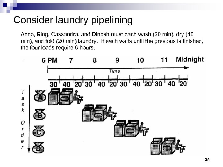Consider laundry pipelining Anne, Bing, Cassandra, and Dinesh must each wash (30 min), dry (40 min), and fold (20 min) laundry. If each waits until the previous is finished, the four loads require 6 hours. 38

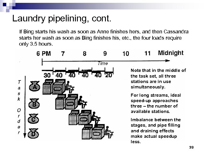Laundry pipelining, cont. If Bing starts his wash as soon as Anne finishes hers, and then Cassandra starts her wash as soon as Bing finishes his, etc. , the four loads require only 3. 5 hours. Note that in the middle of the task set, all three stations are in use simultaneously. For long streams, ideal speed-up approaches three – the number of available stations. Imbalance between the stages, and pipe filling and draining effects make actual speedup less. 39

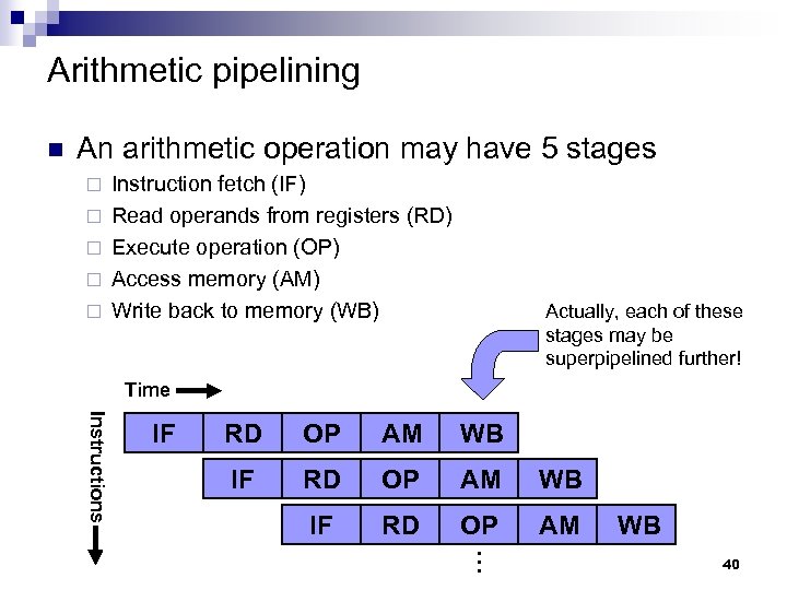Arithmetic pipelining n An arithmetic operation may have 5 stages ¨ ¨ ¨ Instruction fetch (IF) Read operands from registers (RD) Execute operation (OP) Access memory (AM) Write back to memory (WB) Actually, each of these stages may be superpipelined further! Time Instructions IF RD OP AM WB … 40

Benefits of pipelining n n Allows the computer to be physically larger Signals need travel only from one stage to the next per clock cycle, not over entire computer 41

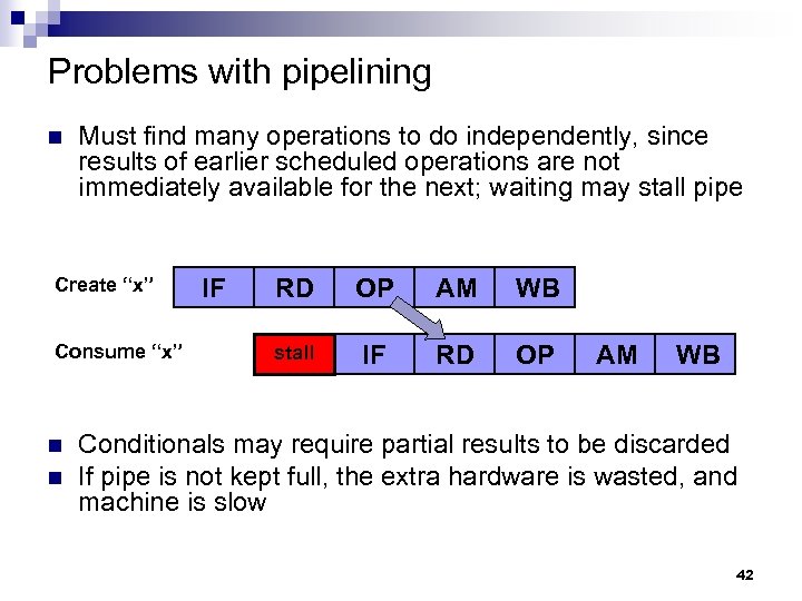Problems with pipelining n Must find many operations to do independently, since results of earlier scheduled operations are not immediately available for the next; waiting may stall pipe Create “x” Consume “x” n n IF RD OP AM WB stall IF RD OP AM WB Conditionals may require partial results to be discarded If pipe is not kept full, the extra hardware is wasted, and machine is slow 42

Parallelism 43

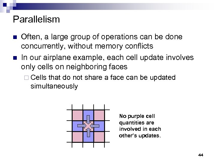Parallelism n n Often, a large group of operations can be done concurrently, without memory conflicts In our airplane example, each cell update involves only cells on neighboring faces ¨ Cells that do not share a face can be updated simultaneously No purple cell quantities are involved in each other’s updates. 44

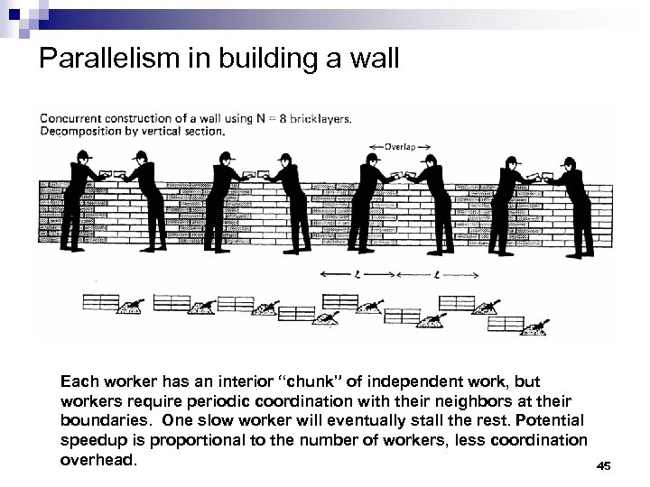Parallelism in building a wall Each worker has an interior “chunk” of independent work, but workers require periodic coordination with their neighbors at their boundaries. One slow worker will eventually stall the rest. Potential speedup is proportional to the number of workers, less coordination overhead. 45

Benefits of parallelism n n n Allows the computer to be physically larger If we had one million computers, then each computer would only have to do 8 x 109 operations per second This would allow the computers to be about 3 cm apart 46

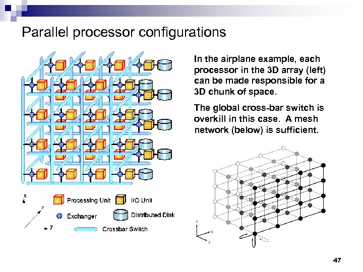Parallel processor configurations In the airplane example, each processor in the 3 D array (left) can be made responsible for a 3 D chunk of space. The global cross-bar switch is overkill in this case. A mesh network (below) is sufficient. 47

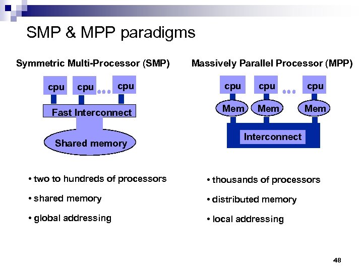SMP & MPP paradigms Symmetric Multi-Processor (SMP) Massively Parallel Processor (MPP) cpu cpu Fast Interconnect Mem Mem cpu Shared memory Interconnect • two to hundreds of processors • thousands of processors • shared memory • distributed memory • global addressing • local addressing 48

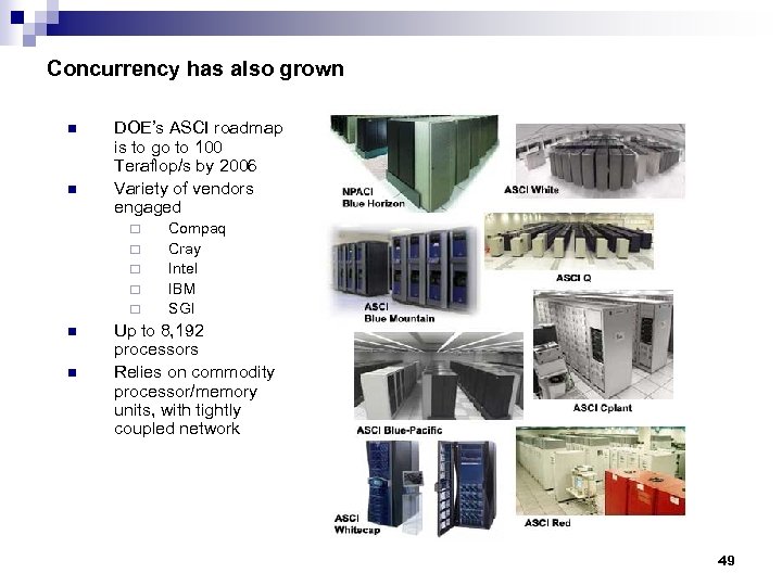Concurrency has also grown n n DOE’s ASCI roadmap is to go to 100 Teraflop/s by 2006 Variety of vendors engaged ¨ ¨ ¨ n n Compaq Cray Intel IBM SGI Up to 8, 192 processors Relies on commodity processor/memory units, with tightly coupled network 49

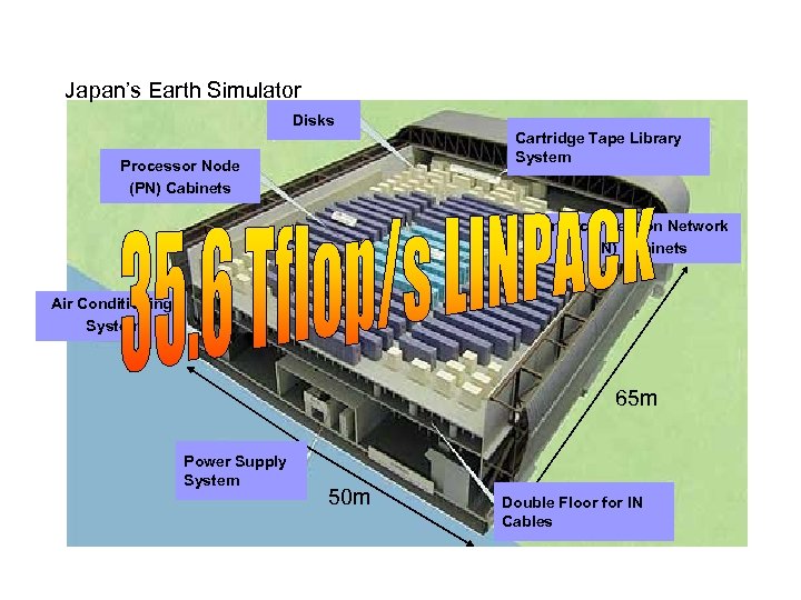Japan’s Earth Simulator of the Earth Simulator System Bird’s-eye View Disks Cartridge Tape Library System Processor Node (PN) Cabinets Interconnection Network (IN) Cabinets Air Conditioning System 65 m Power Supply System 50 m Double Floor for IN Cables 50

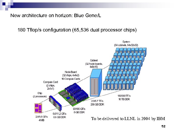New architecture on horizon: Blue Gene/L 180 Tflop/s configuration (65, 536 dual processor chips) To be delivered to LLNL in 2004 by IBM 52

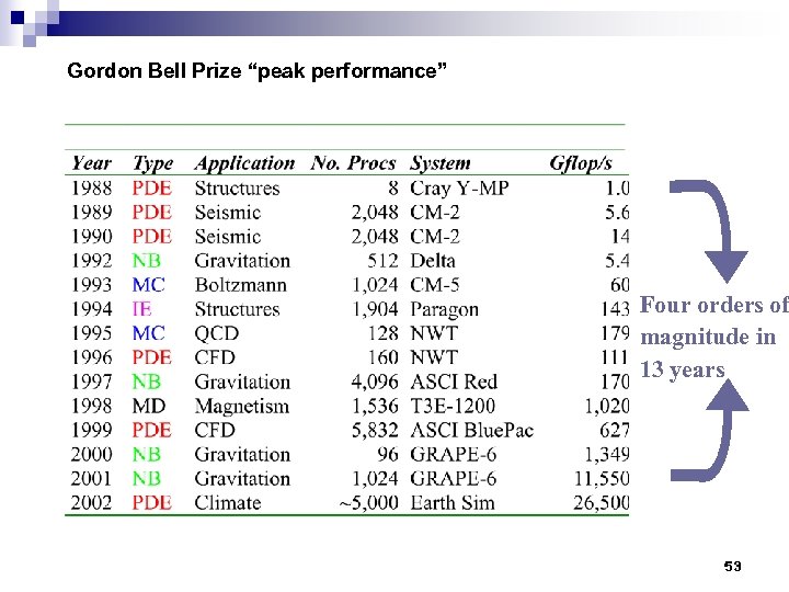Gordon Bell Prize “peak performance” Four orders of magnitude in 13 years 53

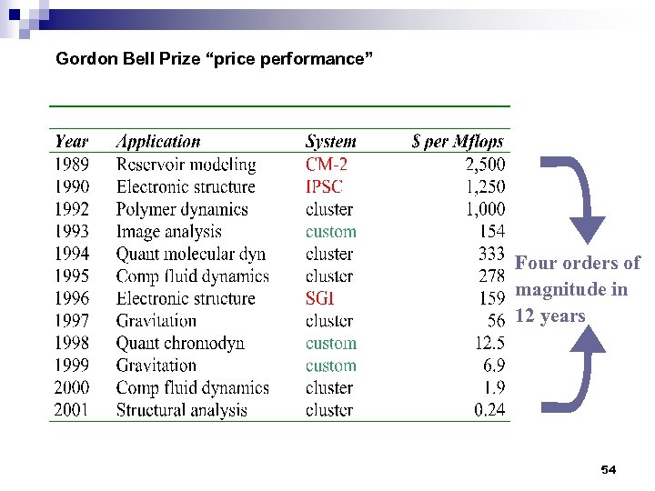Gordon Bell Prize “price performance” Four orders of magnitude in 12 years 54

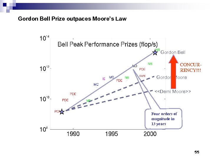Gordon Bell Prize outpaces Moore’s Law Gordon Bell CONCURRENCY!!! Gordon Moore <> Four orders of magnitude in 13 years 55

Problems with parallelism n n Must find massive concurrency in the task Still need many computers, each of which must be fast Communication between computers becomes a dominant factor Amdahl’s Law limits speedup available based on remaining non-concurrent work 56

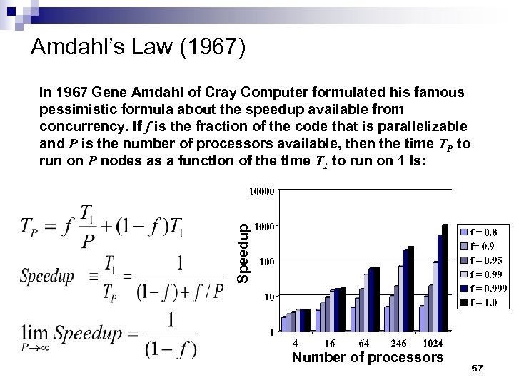Amdahl’s Law (1967) Speedup In 1967 Gene Amdahl of Cray Computer formulated his famous pessimistic formula about the speedup available from concurrency. If f is the fraction of the code that is parallelizable and P is the number of processors available, then the time TP to run on P nodes as a function of the time T 1 to run on 1 is: Number of processors 57

Algorithms 58

Algorithms are key “I would rather have today’s algorithms on yesterday’s computers than vice versa. ” Philippe Toint 59

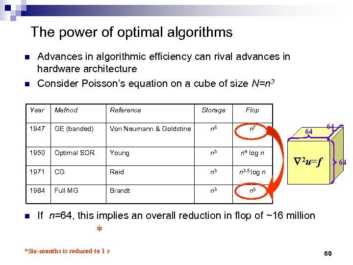The power of optimal algorithms n n Advances in algorithmic efficiency can rival advances in hardware architecture Consider Poisson’s equation on a cube of size N=n 3 Year Method Reference Storage Flop 1947 GE (banded) Von Neumann & Goldstine n 5 n 7 1950 Optimal SOR Young n 3 n 4 log n n 3. 5 log 1971 CG Reid n 3 1984 Full MG Brandt n 3 n 64 64 2 u=f 64 n n 3 If n=64, this implies an overall reduction in flop of ~16 million * *Six-months is reduced to 1 s 60

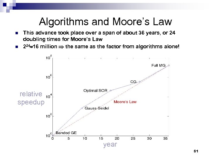Algorithms and Moore’s Law n n This advance took place over a span of about 36 years, or 24 doubling times for Moore’s Law 224 16 million the same as the factor from algorithms alone! relative speedup year 61

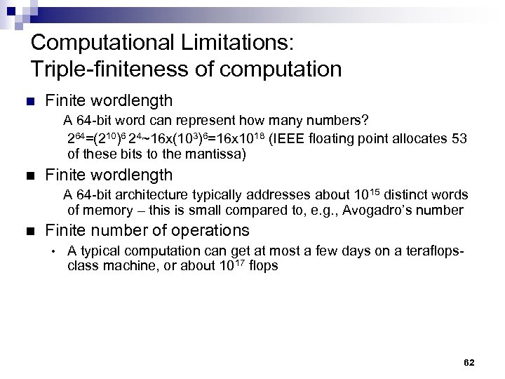Computational Limitations: Triple-finiteness of computation n Finite wordlength A 64 -bit word can represent how many numbers? 264=(210)6 24~16 x(103)6=16 x 1018 (IEEE floating point allocates 53 of these bits to the mantissa) n Finite wordlength A 64 -bit architecture typically addresses about 1015 distinct words of memory – this is small compared to, e. g. , Avogadro’s number n Finite number of operations • A typical computation can get at most a few days on a teraflopsclass machine, or about 1017 flops 62

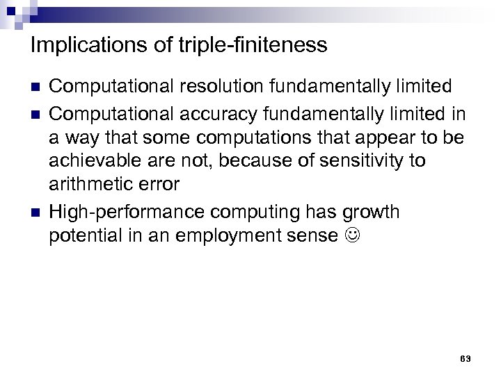Implications of triple-finiteness n n n Computational resolution fundamentally limited Computational accuracy fundamentally limited in a way that some computations that appear to be achievable are not, because of sensitivity to arithmetic error High-performance computing has growth potential in an employment sense 63

Computational Difficulties: Conditioning, accuracy, stability n Problem is ill-conditioned if a small change in the input data can make a large change in the output ¨ ¨ n Process is unstable if the result it produces is sensitive to floating point errors made during its execution ¨ ¨ n characteristic of the process, not of the problem another algorithm may help Only if a stable algorithm is applied to a well-conditioned problem may an accurate result be expected ¨ n characteristic of the problem, not of the process in severe cases, no algorithm can help If either stability or accuracy is missing the computation may be a waste of time and the result misleading We avoid at present the subject of nonuniqueness ¨ Important in nonlinear problems 64

Applications 65

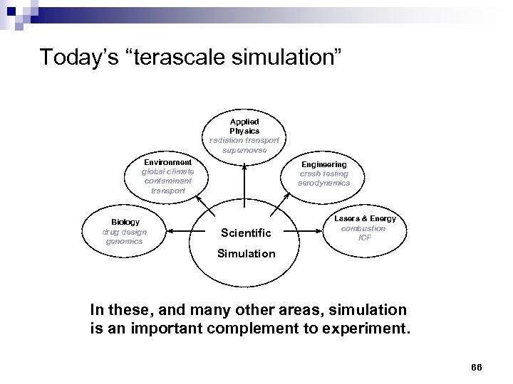Today’s “terascale simulation” Applied Physics radiation transport supernovae Environment global climate contaminant transport Biology drug design genomics Engineering crash testing aerodynamics Scientific Lasers & Energy combustion ICF Simulation In these, and many other areas, simulation is an important complement to experiment. 66

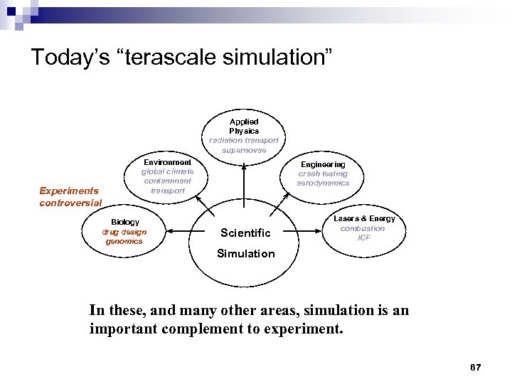Today’s “terascale simulation” Applied Physics radiation transport supernovae Experiments controversial Environment global climate contaminant transport Biology drug design genomics Engineering crash testing aerodynamics Scientific Lasers & Energy combustion ICF Simulation In these, and many other areas, simulation is an important complement to experiment. 67

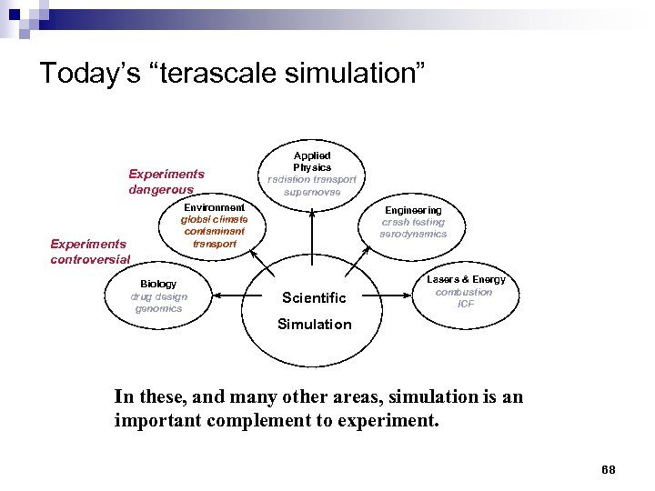Today’s “terascale simulation” Experiments dangerous Experiments controversial Applied Physics radiation transport supernovae Environment global climate contaminant transport Biology drug design genomics Engineering crash testing aerodynamics Scientific Lasers & Energy combustion ICF Simulation In these, and many other areas, simulation is an important complement to experiment. 68

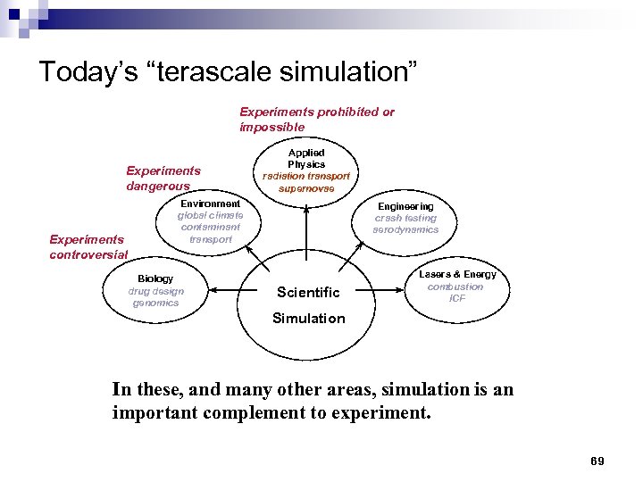Today’s “terascale simulation” Experiments prohibited or impossible Experiments dangerous Experiments controversial Applied Physics radiation transport supernovae Environment global climate contaminant transport Biology drug design genomics Engineering crash testing aerodynamics Scientific Lasers & Energy combustion ICF Simulation In these, and many other areas, simulation is an important complement to experiment. 69

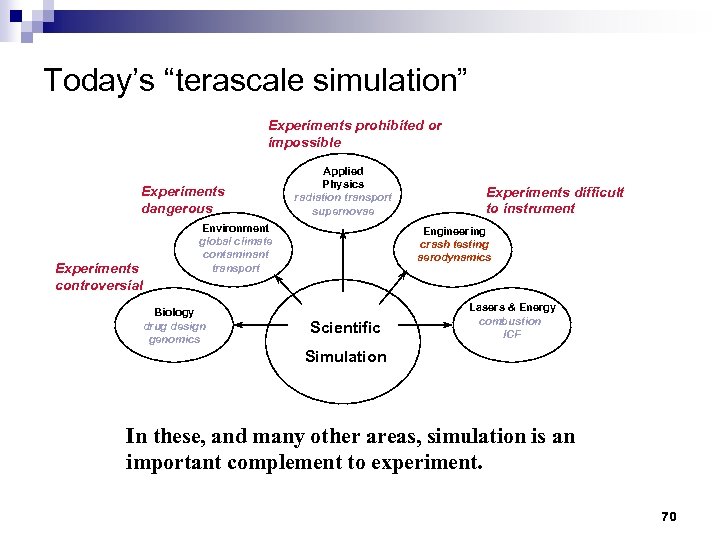Today’s “terascale simulation” Experiments prohibited or impossible Experiments dangerous Experiments controversial Applied Physics radiation transport supernovae Environment global climate contaminant transport Biology drug design genomics Experiments difficult to instrument Engineering crash testing aerodynamics Scientific Lasers & Energy combustion ICF Simulation In these, and many other areas, simulation is an important complement to experiment. 70

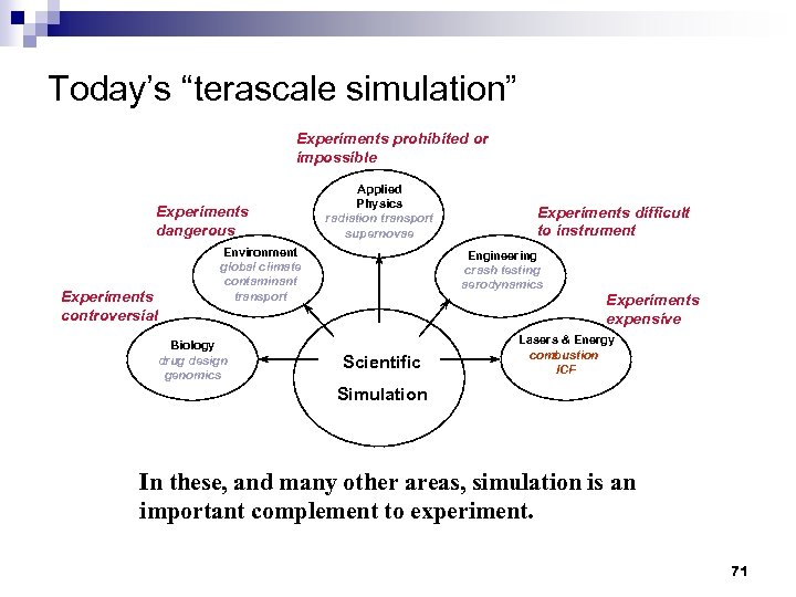Today’s “terascale simulation” Experiments prohibited or impossible Experiments dangerous Experiments controversial Applied Physics radiation transport supernovae Environment global climate contaminant transport Biology drug design genomics Experiments difficult to instrument Engineering crash testing aerodynamics Experiments expensive Scientific Lasers & Energy combustion ICF Simulation In these, and many other areas, simulation is an important complement to experiment. 71

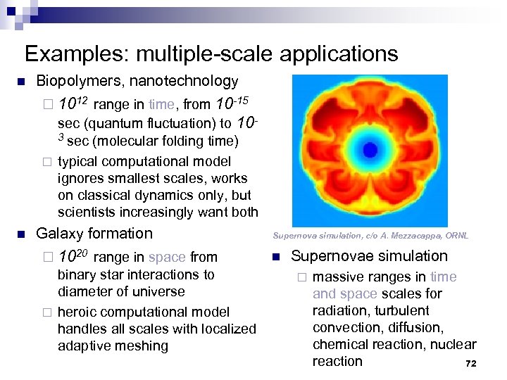Examples: multiple-scale applications n Biopolymers, nanotechnology ¨ 1012 range in time, from 10 -15 sec (quantum fluctuation) to 103 sec (molecular folding time) ¨ typical computational model ignores smallest scales, works on classical dynamics only, but scientists increasingly want both n Galaxy formation ¨ 1020 range in space from binary star interactions to diameter of universe ¨ heroic computational model handles all scales with localized adaptive meshing Supernova simulation, c/o A. Mezzacappa, ORNL n Supernovae simulation ¨ massive ranges in time and space scales for radiation, turbulent convection, diffusion, chemical reaction, nuclear reaction 72

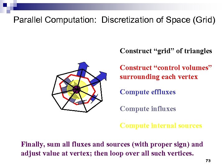Parallel Computation: Discretization of Space (Grid) Construct “grid” of triangles Construct “control volumes” surrounding each vertex Compute effluxes Compute internal sources Finally, sum all fluxes and sources (with proper sign) and adjust value at vertex; then loop over all such vertices. 73

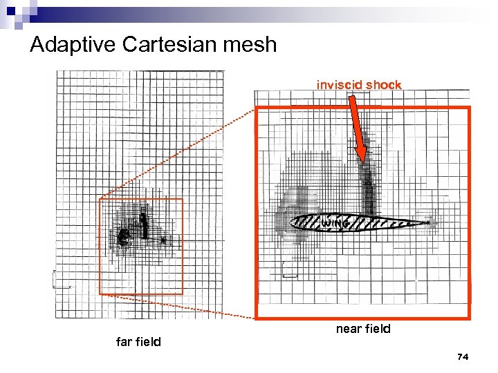Adaptive Cartesian mesh inviscid shock far field near field 74

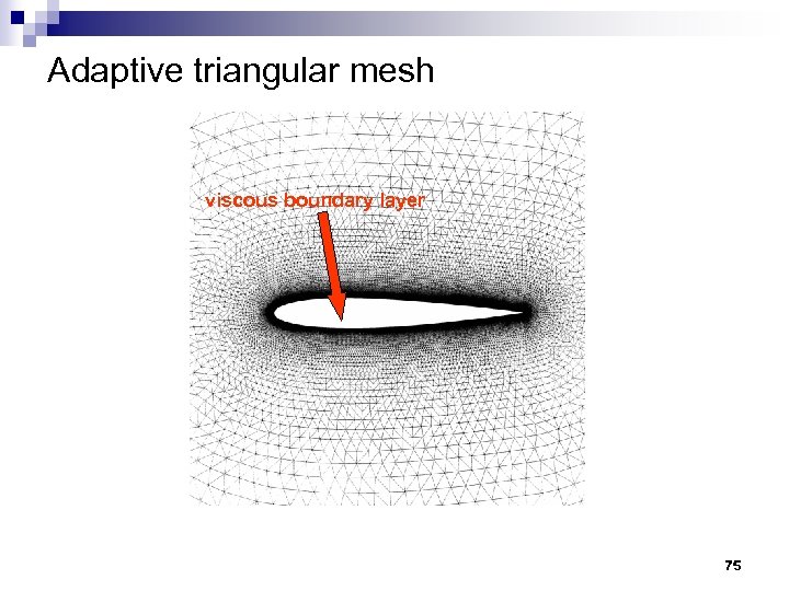Adaptive triangular mesh viscous boundary layer 75

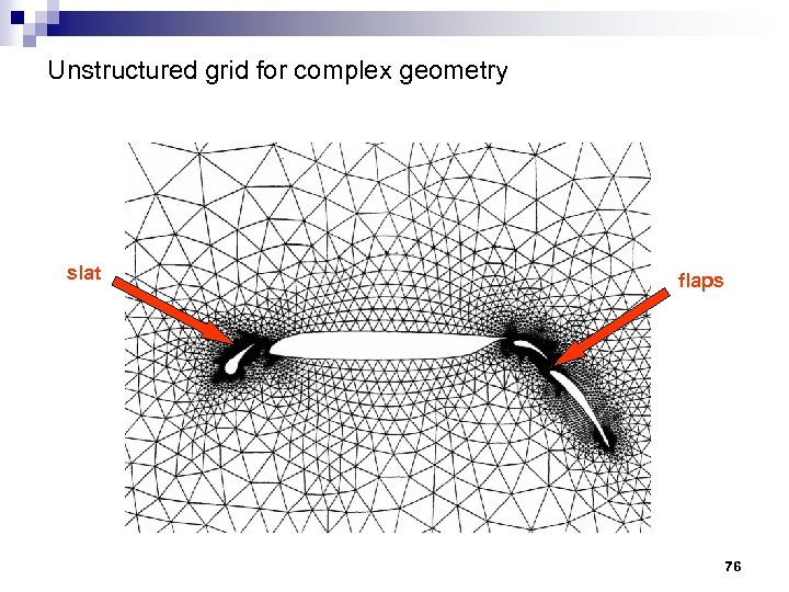Unstructured grid for complex geometry slat flaps 76

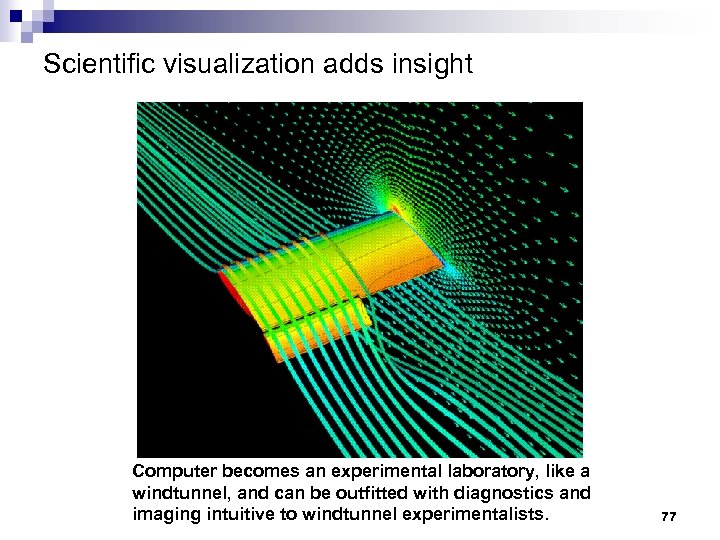Scientific visualization adds insight Computer becomes an experimental laboratory, like a windtunnel, and can be outfitted with diagnostics and imaging intuitive to windtunnel experimentalists. 77

What would scientists do with 100 -1000 x? Example: predicting future climates n Resolution refine horizontal from 160 to 40 km ¨ refine vertical from 105 to 15 km ¨ n New physics atmospheric chemistry ¨ carbon cycle ¨ dynamic terrestrial vegetation (nitrogen and sulfur cycles and landuse and land-cover changes) ¨ n Improved representation of subgrid processes clouds ¨ atmospheric radiative transfer ¨ 78

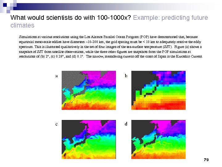What would scientists do with 100 -1000 x? Example: predicting future climates Simulations at various resolutions using the Los Alamos Parallel Ocean Program (POP) have demonstrated that, because equatorial meso-scale eddies have diameters ~10 -200 km, the grid spacing must be < 10 km to adequately resolve the eddy spectrum. This is illustrated qualitatively in the set of four images of the sea-surface temperature (SST). Figure (a) shows a snapshot of SST from satellite observations, while three other figures are snapshots from the POP simulations at resolutions of (b) 2 , (c) 0. 28 , and (d) 0. 1. The narrow, meandering current off the coast of Japan is the Kuroshio Current 79

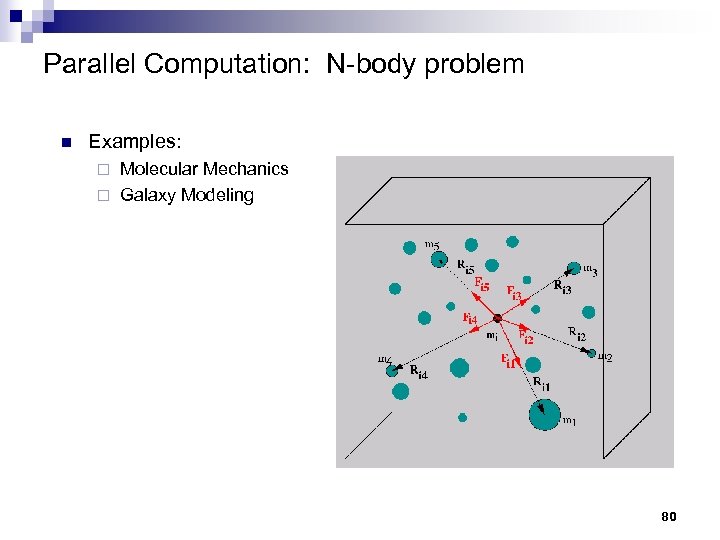Parallel Computation: N-body problem n Examples: Molecular Mechanics ¨ Galaxy Modeling ¨ 80