Computer Graphics using Open GL 3 rd Edition

Computer Graphics using Open. GL, 3 rd Edition F. S. Hill, Jr. and S. Kelley Chapter 5. 1 -2 Transformations of Objects S. M. Lea University of North Carolina at Greensboro © 2007, Prentice Hall

Transformations • We used the window to viewport transformation to scale and translate objects in the world window to their size and position in the viewport. • We want to build on this idea, and gain more flexible control over the size, orientation, and position of objects of interest. • To do so, we will use the powerful affine transformation.

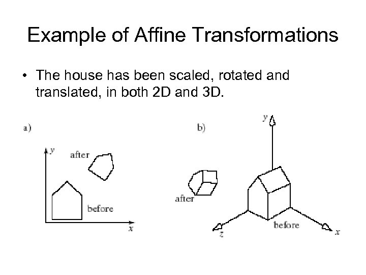Example of Affine Transformations • The house has been scaled, rotated and translated, in both 2 D and 3 D.

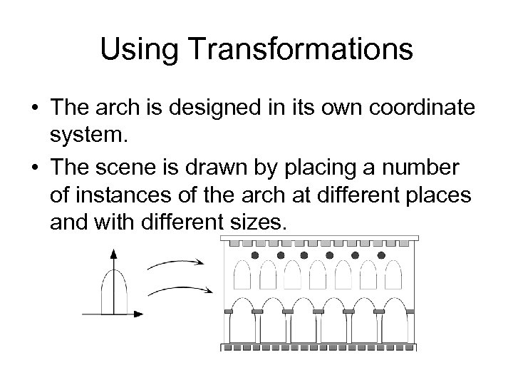Using Transformations • The arch is designed in its own coordinate system. • The scene is drawn by placing a number of instances of the arch at different places and with different sizes.

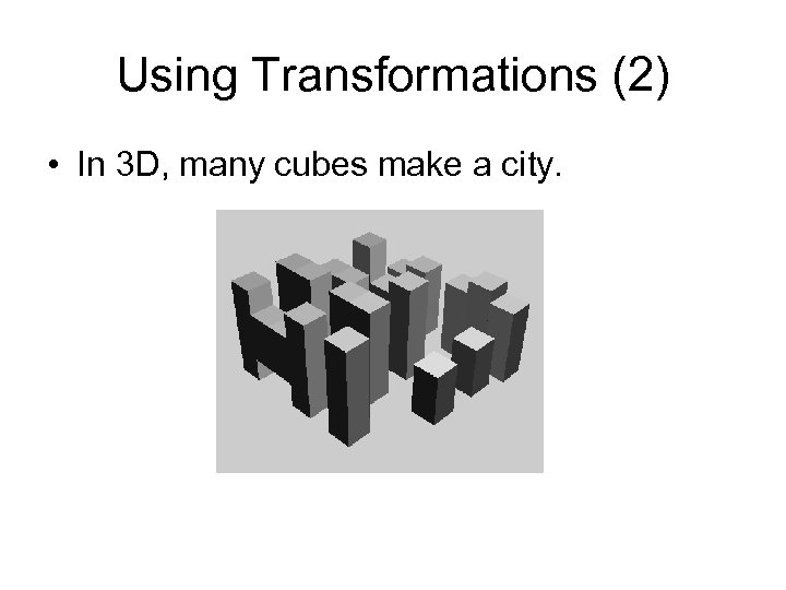Using Transformations (2) • In 3 D, many cubes make a city.

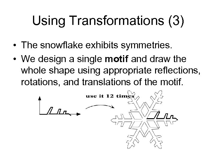Using Transformations (3) • The snowflake exhibits symmetries. • We design a single motif and draw the whole shape using appropriate reflections, rotations, and translations of the motif.

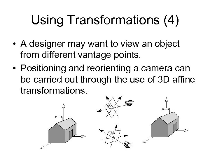Using Transformations (4) • A designer may want to view an object from different vantage points. • Positioning and reorienting a camera can be carried out through the use of 3 D affine transformations.

Using Transformations (5) • In a computer animation, objects move. • We make them move by translating and rotating their local coordinate systems as the animation proceeds. • A number of graphics platforms, including Open. GL, provide a graphics pipeline: a sequence of operations which are applied to all points that are sent through it. • A drawing is produced by processing each point.

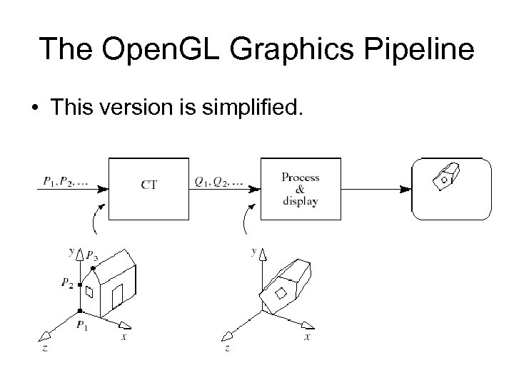The Open. GL Graphics Pipeline • This version is simplified.

Graphics Pipeline (2) • An application sends the pipeline a sequence of points P 1, P 2, . . . using commands such as: gl. Begin(GL_LINES); gl. Vertex 3 f(. . . ); // send P 1 through the pipeline gl. Vertex 3 f(. . . ); // send P 2 through the pipeline. . . gl. End(); • These points first encounter a transformation called the current transformation (CT), which alters their values into a different set of points, say Q 1, Q 2, Q 3.

Graphics Pipeline (3) • Just as the original points Pi describe some geometric object, the points Qi describe the transformed version of the same object. • These points are then sent through additional steps, and ultimately are used to draw the final image on the display.

Graphics Pipeline (4) • Prior to Open. GL 2. 0 the pipeline was of fixedfunctionality: each stage had to perform a specific operation in a particular manner. • With Open. GL 2. 0 and the Shading Language (GLSL), the application programmer could not only change the order in which some operations were performed, but in addition could make the operations programmable. • This allows hardware and software developers to take advantage of new algorithms and rendering techniques and still comply with Open. GL version 2. 0.

Transformations • Transformations change 2 D or 3 D points and vectors, or change coordinate systems. – An object transformation alters the coordinates of each point on the object according to the same rule, leaving the underlying coordinate system fixed. – A coordinate transformation defines a new coordinate system in terms of the old one, then represents all of the object’s points in this new system. • Object transformations are easier to understand, so we will do them first.

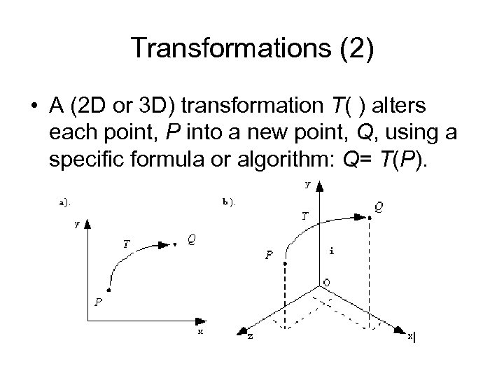Transformations (2) • A (2 D or 3 D) transformation T( ) alters each point, P into a new point, Q, using a specific formula or algorithm: Q= T(P).

Transformations (3) • An arbitrary point P in the plane is mapped to Q. • Q is the image of P under the mapping T. • We transform an object by transforming each of its points, using the same function T() for each point. • The image of line L under T, for instance, consists of the images of all the individual points of L.

Transformations (4) • Most mappings of interest are continuous, so the image of a straight line is still a connected curve of some shape, although it’s not necessarily a straight line. • Affine transformations, however, do preserve lines: the image under T of a straight line is also a straight line.

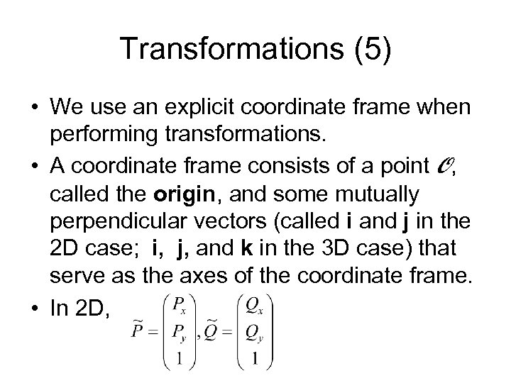Transformations (5) • We use an explicit coordinate frame when performing transformations. • A coordinate frame consists of a point O, called the origin, and some mutually perpendicular vectors (called i and j in the 2 D case; i, j, and k in the 3 D case) that serve as the axes of the coordinate frame. • In 2 D,

Transformations (6) • Recall that this means that point P is at location = Px i + Py j + O , and similarly for Q. • Px and Py are the coordinates of P. • To get from the origin to point P, move amount Px along axis i and amount Py along axis j.

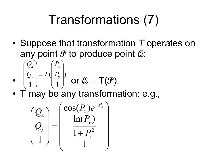Transformations (7) • Suppose that transformation T operates on any point P to produce point Q: • or Q = T(P). • T may be any transformation: e. g. ,

Transformations (8) • To make affine transformations we restrict ourselves to much simpler families of functions, those that are linear in Px and Py. • Affine transformations make it easy to scale, rotate, and reposition figures. • Successive affine transformations can be combined into a single overall affine transformation.

Affine Transformations • Affine transformations have a compact matrix representation. • The matrix associated with an affine transformation operating on 2 D vectors or points must be a three-by-three matrix. – This is a direct consequence of representing the vectors and points in homogeneous coordinates.

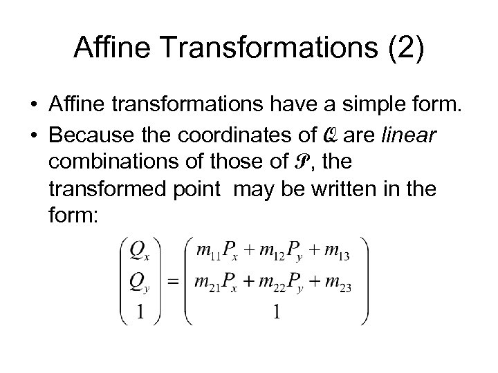Affine Transformations (2) • Affine transformations have a simple form. • Because the coordinates of Q are linear combinations of those of P, the transformed point may be written in the form:

Affine Transformations (3) • There are six given constants: m 11, m 12, etc. • The coordinate Qx consists of portions of both Px and Py, and so does Qy. • This combination between the x- and ycomponents also gives rise to rotations and shears.

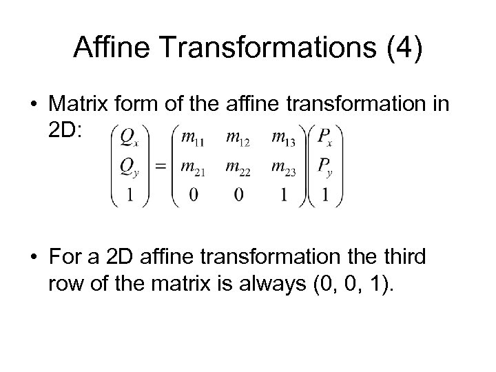Affine Transformations (4) • Matrix form of the affine transformation in 2 D: • For a 2 D affine transformation the third row of the matrix is always (0, 0, 1).

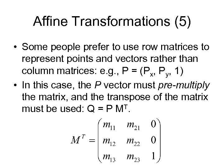Affine Transformations (5) • Some people prefer to use row matrices to represent points and vectors rather than column matrices: e. g. , P = (Px, Py, 1) • In this case, the P vector must pre-multiply the matrix, and the transpose of the matrix must be used: Q = P MT.

Affine Transformations (6) • Vectors can be transformed as well as points. • If a 2 D vector v has coordinates Vx and Vy then its coordinate frame representation is a column vector with third component 0.

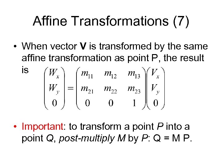Affine Transformations (7) • When vector V is transformed by the same affine transformation as point P, the result is • Important: to transform a point P into a point Q, post-multiply M by P: Q = M P.

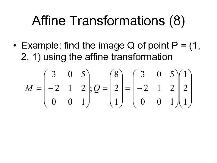Affine Transformations (8) • Example: find the image Q of point P = (1, 2, 1) using the affine transformation

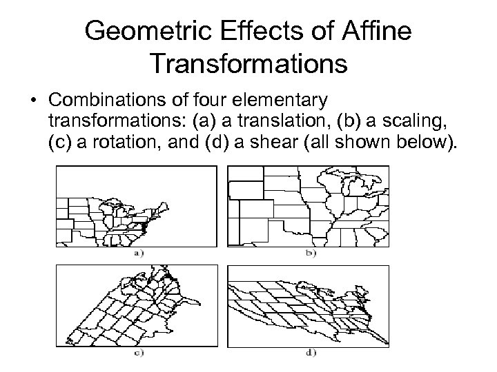Geometric Effects of Affine Transformations • Combinations of four elementary transformations: (a) a translation, (b) a scaling, (c) a rotation, and (d) a shear (all shown below).

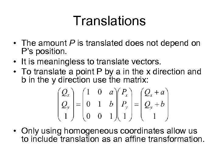Translations • The amount P is translated does not depend on P’s position. • It is meaningless to translate vectors. • To translate a point P by a in the x direction and b in the y direction use the matrix: • Only using homogeneous coordinates allow us to include translation as an affine transformation.

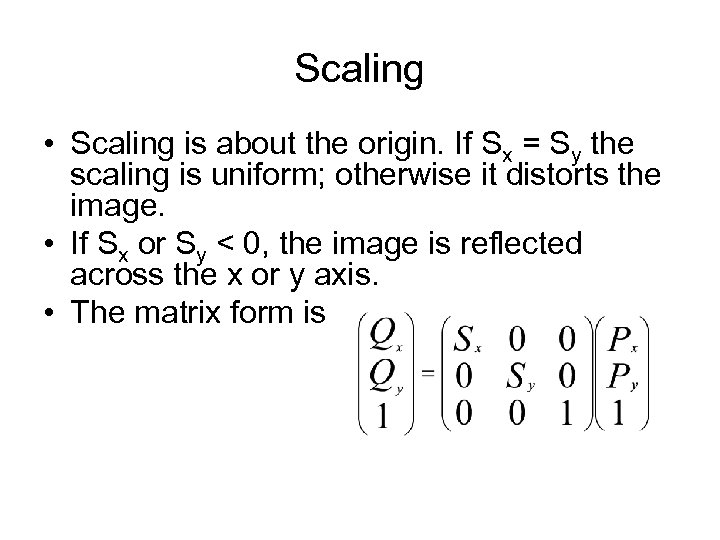Scaling • Scaling is about the origin. If Sx = Sy the scaling is uniform; otherwise it distorts the image. • If Sx or Sy < 0, the image is reflected across the x or y axis. • The matrix form is

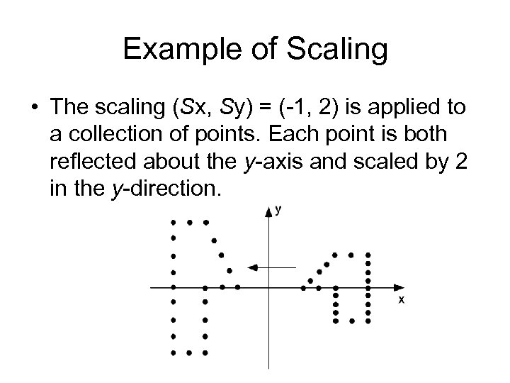Example of Scaling • The scaling (Sx, Sy) = (-1, 2) is applied to a collection of points. Each point is both reflected about the y-axis and scaled by 2 in the y-direction.

Types of Scaling • Pure reflections, for which each of the scale factors is +1 or -1. • A uniform scaling, or a magnification about the origin: Sx = Sy, magnification |S|. – Reflection also occurs if Sx or Sy is negative. – If |S| < 1, the points will be moved closer to the origin, producing a reduced image. • If the scale factors are not the same, the scaling is called a differential scaling.

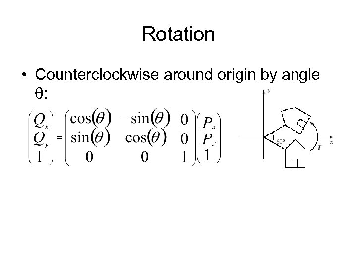Rotation • Counterclockwise around origin by angle θ:

Deriving the Rotation Matrix • P is at distance R from the origin, at angle Φ; then P = (R cos(Φ), R sin(Φ)). • Q must be at the same distance as P, and at angle θ + Φ: Q =(R cos(θ + Φ), R sin(θ + Φ)). • cos(θ + Φ) = cos(θ) cos(Φ) - sin(θ) sin(Φ); sin(θ + Φ) = sin(θ) cos(Φ) + cos(θ) sin(Φ). • Use Px = R cos(Φ) and Py = R sin(Φ).

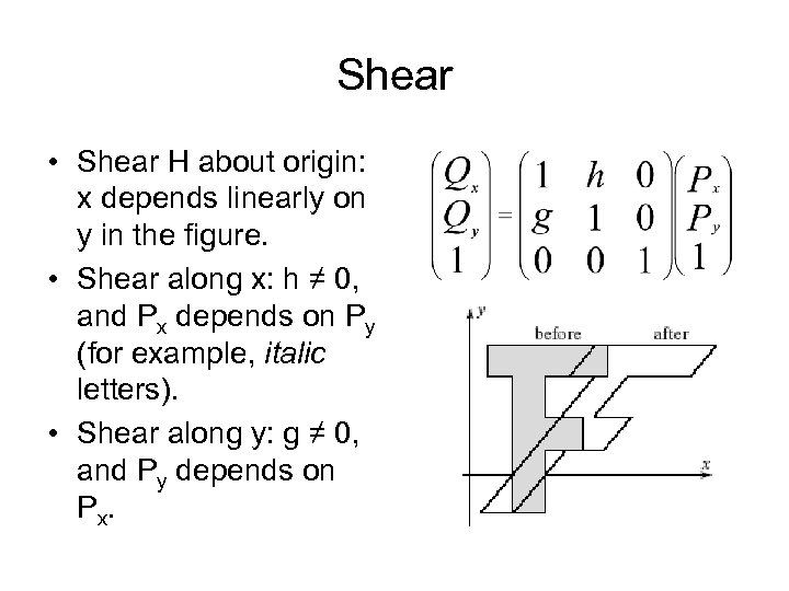Shear • Shear H about origin: x depends linearly on y in the figure. • Shear along x: h ≠ 0, and Px depends on Py (for example, italic letters). • Shear along y: g ≠ 0, and Py depends on Px.

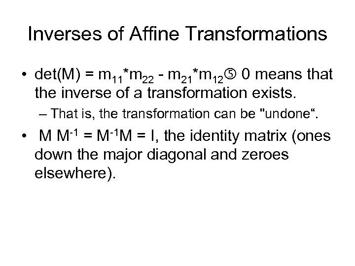Inverses of Affine Transformations • det(M) = m 11*m 22 - m 21*m 12 0 means that the inverse of a transformation exists. – That is, the transformation can be "undone“. • M M-1 = M-1 M = I, the identity matrix (ones down the major diagonal and zeroes elsewhere).

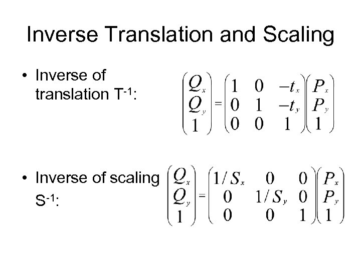Inverse Translation and Scaling • Inverse of translation T-1: • Inverse of scaling S-1:

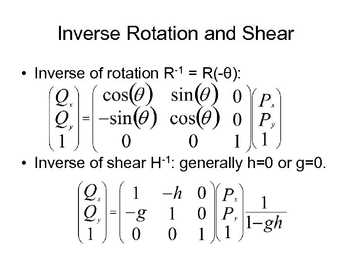Inverse Rotation and Shear • Inverse of rotation R-1 = R(-θ): • Inverse of shear H-1: generally h=0 or g=0.

Composing Affine Transformations • Usually, we want to apply several affine transformations in a particular order to the figures in a scene: for example, – translate by (3, - 4) – then rotate by 30 o – then scale by (2, - 1) and so on. • Applying successive affine transformations is called composing affine transformations.

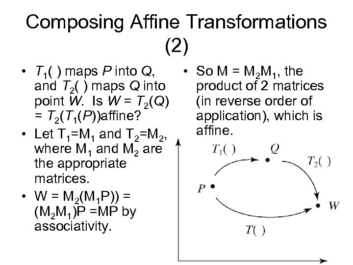Composing Affine Transformations (2) • T 1( ) maps P into Q, and T 2( ) maps Q into point W. Is W = T 2(Q) = T 2(T 1(P))affine? • Let T 1=M 1 and T 2=M 2, where M 1 and M 2 are the appropriate matrices. • W = M 2(M 1 P)) = (M 2 M 1)P =MP by associativity. • So M = M 2 M 1, the product of 2 matrices (in reverse order of application), which is affine.

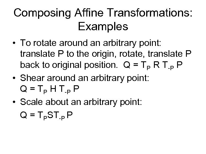Composing Affine Transformations: Examples • To rotate around an arbitrary point: translate P to the origin, rotate, translate P back to original position. Q = TP R T-P P • Shear around an arbitrary point: Q = TP H T-P P • Scale about an arbitrary point: Q = TPST-P P

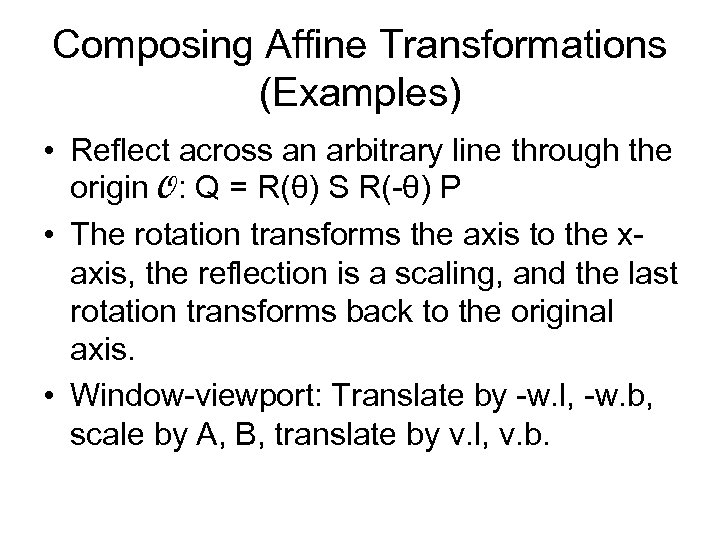Composing Affine Transformations (Examples) • Reflect across an arbitrary line through the origin O: Q = R(θ) S R(-θ) P • The rotation transforms the axis to the xaxis, the reflection is a scaling, and the last rotation transforms back to the original axis. • Window-viewport: Translate by -w. l, -w. b, scale by A, B, translate by v. l, v. b.

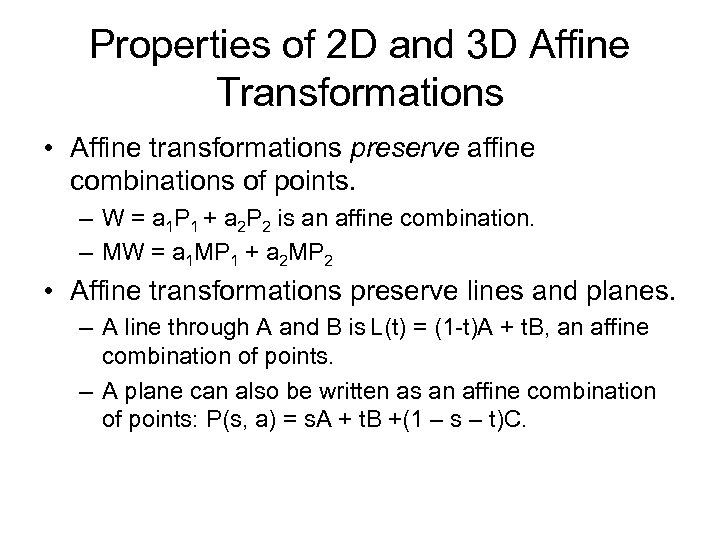Properties of 2 D and 3 D Affine Transformations • Affine transformations preserve affine combinations of points. – W = a 1 P 1 + a 2 P 2 is an affine combination. – MW = a 1 MP 1 + a 2 MP 2 • Affine transformations preserve lines and planes. – A line through A and B is L(t) = (1 -t)A + t. B, an affine combination of points. – A plane can also be written as an affine combination of points: P(s, a) = s. A + t. B +(1 – s – t)C.

Properties of Transformations (2) • Parallelism of lines and planes is preserved. – Line A + bt having direction b transforms to the line given in homogeneous coordinates by M(A + bt) = MA + Mbt, which has direction vector Mb. – Mb does not depend on point A. Thus two different lines A 1+ bt and A 2 + bt that have the same direction will transform into two lines both having the direction, so they are parallel. • An important consequence of this property is that parallelograms map into other parallelograms.

Properties of Transformations (3) • The direction vectors for a plane also transform into new direction vectors independent of the location of the plane. • As a consequence, parallelepipeds map into other parallelepipeds.

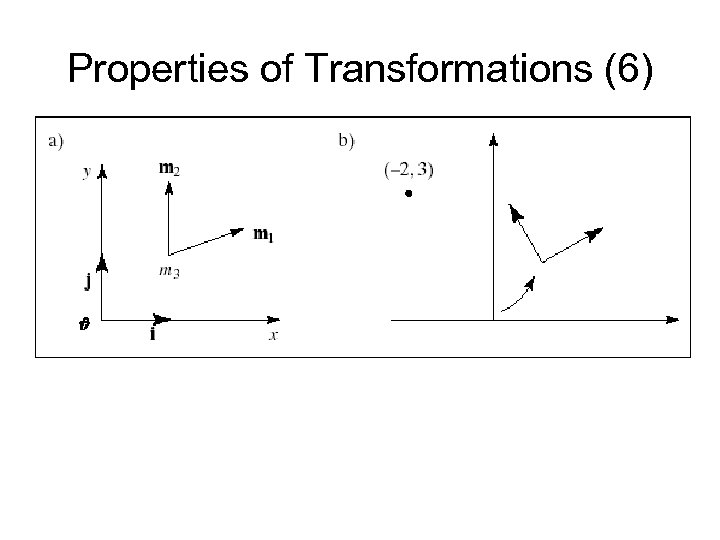
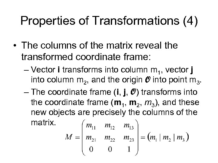Properties of Transformations (4) • The columns of the matrix reveal the transformed coordinate frame: – Vector i transforms into column m 1, vector j into column m 2, and the origin O into point m 3. – The coordinate frame (i, j, O) transforms into the coordinate frame (m 1, m 2, m 3), and these new objects are precisely the columns of the matrix.

Properties of Transformations (5) • The axes of the new coordinate frame are not necessarily perpendicular, nor must they be unit length. – They are still perpendicular if the transformation involves only rotations and uniform scalings. • Any point P = Pxi + Pyj + O transforms into Q = Pxm 1 + Pym 2 + m 3.

Properties of Transformations (6)

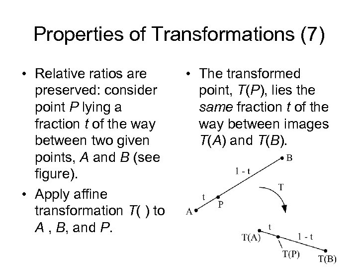Properties of Transformations (7) • Relative ratios are preserved: consider point P lying a fraction t of the way between two given points, A and B (see figure). • Apply affine transformation T( ) to A , B, and P. • The transformed point, T(P), lies the same fraction t of the way between images T(A) and T(B).

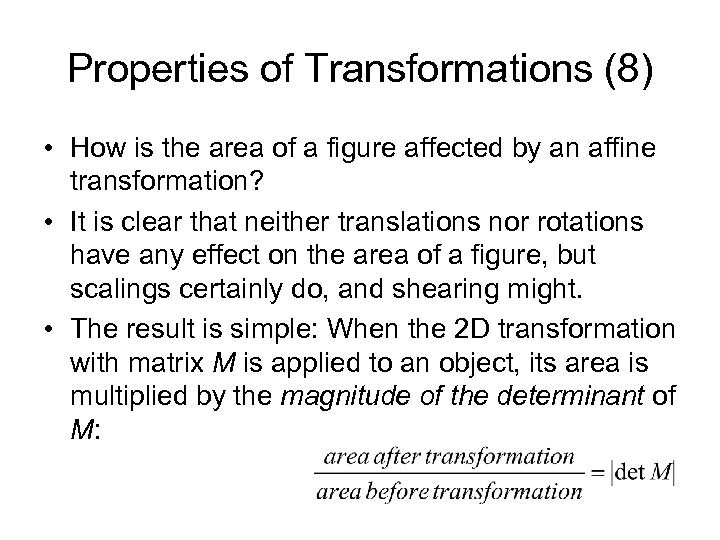Properties of Transformations (8) • How is the area of a figure affected by an affine transformation? • It is clear that neither translations nor rotations have any effect on the area of a figure, but scalings certainly do, and shearing might. • The result is simple: When the 2 D transformation with matrix M is applied to an object, its area is multiplied by the magnitude of the determinant of M:

Properties of Transformations (9) • In 2 D the determinant of the matrix M is (m 11 m 22 – m 12 m 21). • For a pure scaling, the new area is Sx. Sy times the original area, whereas for a shear along one axis the new area is the same as the original area. • In 3 D similar arguments apply, and we can conclude that the volume of a 3 D object is scaled by |det M| when the object is transformed by the 3 D transformation based on matrix M.

Properties of Transformations (10) • Every affine transformation is composed of elementary operations. • A matrix may be factored into a product of elementary matrices in various ways. One particular way of factoring the matrix associated with a 2 D affine transformation yields M = (shear)(scaling)(rotation)(translation) • That is, any 3 x 3 matrix that represents a 2 D affine transformation can be written as the product of (reading right to left) a translation matrix, a rotation matrix, a scaling matrix, and a shear matrix.