Computer Graphics International IT University Administrivia Grading

Computer Graphics International IT University

Administrivia Grading: Assignments: 20% (4 assignments 5% each) Tutorial Exercises: 20% (10 exercises 2% each) Midterm exam: 10% Endterm exam: 10% Final exam 40% Textbook: Fundamentals of Computer Graphics

Course Topics Lectures Theoretical and practical foundations of CG Fundamentals of computer graphics algorithms Assignments & tutorials Experience with Open. GL (industry-standard CG library) Creating realistic 3 D models Creating CG scenes Experience with Open. CV (Open Computer Vision Library)

Introduction What is Computer Graphics?

Computer Graphics is NOT: Learning how to use Photoshop, Corel. Draw and other painting tools. About Graphics Hardware

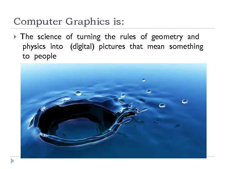Computer Graphics is: The science of turning the rules of geometry and physics into (digital) pictures that mean something to people

Computer Graphics is: The science of turning the rules of geometry and physics into (digital) pictures that mean something to people Technology for generation of visual media (images & digital video) with control over style, appearance, realism, motion, . . . Key Elements: modeling objects & scenes, animation, rendering algorithms & data structures interface design & programming mathematics, physics, optics, psychophysics

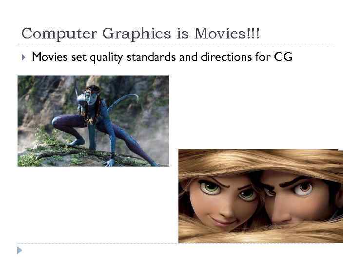Computer Graphics is Movies!!! Movies set quality standards and directions for CG

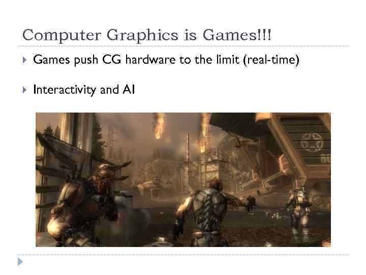Computer Graphics is Games!!! Games push CG hardware to the limit (real-time) Interactivity and AI

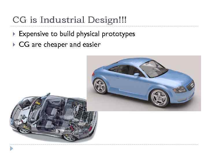CG is Industrial Design!!! Expensive to build physical prototypes CG are cheaper and easier

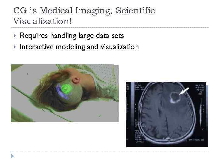CG is Medical Imaging, Scientific Visualization! Requires handling large data sets Interactive modeling and visualization

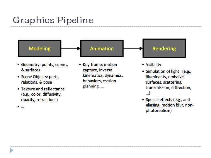Graphics Pipeline

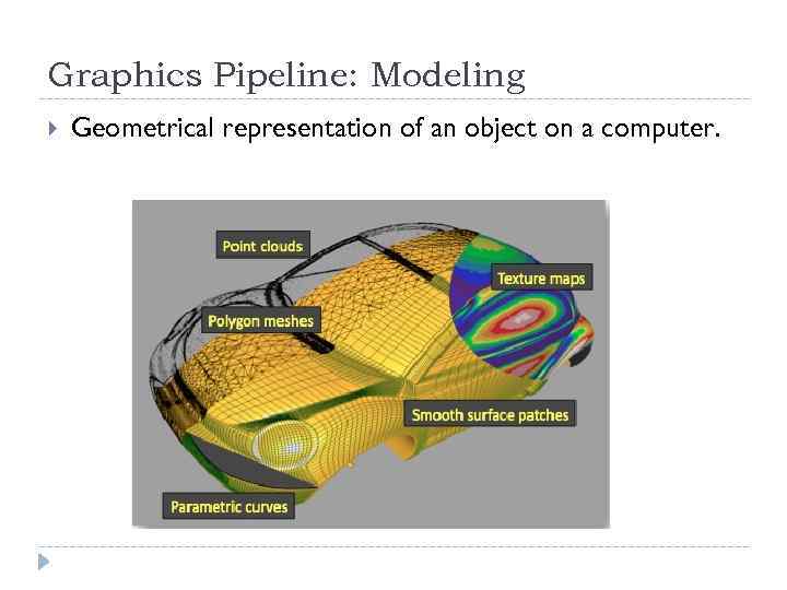Graphics Pipeline: Modeling Geometrical representation of an object on a computer.

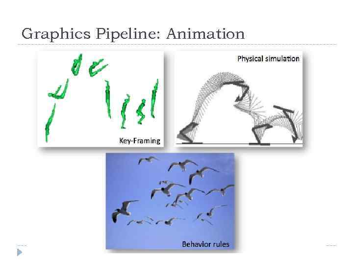Graphics Pipeline: Animation

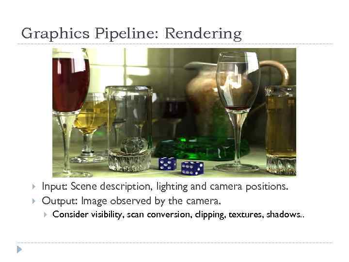Graphics Pipeline: Rendering Input: Scene description, lighting and camera positions. Output: Image observed by the camera. Consider visibility, scan conversion, clipping, textures, shadows. .

Topic 0. A little recap of some MATH Vectors (direction, length) Dot product Cross product

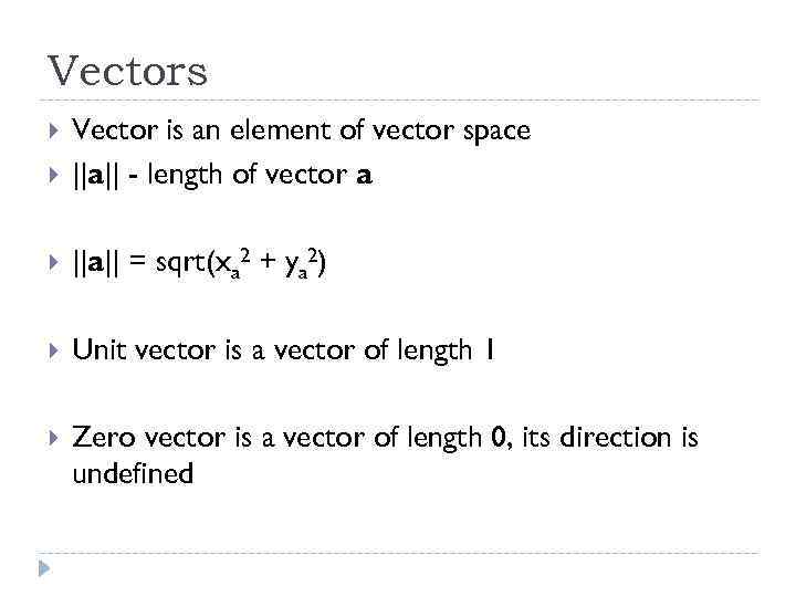Vectors Vector is an element of vector space ||a|| - length of vector a ||a|| = sqrt(xa 2 + ya 2) Unit vector is a vector of length 1 Zero vector is a vector of length 0, its direction is undefined

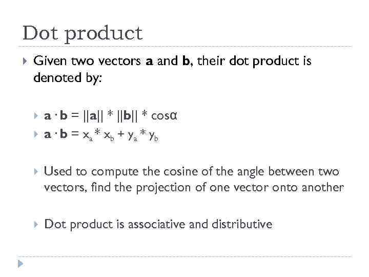Dot product Given two vectors a and b, their dot product is denoted by: a. b = ||a|| * ||b|| * cosα a. b = xa * xb + ya * yb Used to compute the cosine of the angle between two vectors, find the projection of one vector onto another Dot product is associative and distributive

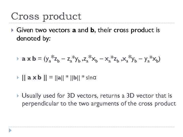Cross product Given two vectors a and b, their cross product is denoted by: a x b = (ya*zb – za*yb , za*xb – xa*zb , xa*yb – ya*xb) || a x b || = ||a|| * ||b|| * sinα Usually used for 3 D vectors, returns a 3 D vector that is perpendicular to the two arguments of the cross product

Topic 1. 2 D Curve representations Explicit representation Parametric representation Tangent & normal vectors Implicit representation

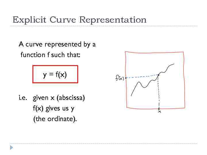Explicit Curve Representation A curve represented by a function f such that: y = f(x) i. e. given x (abscissa) f(x) gives us y (the ordinate).

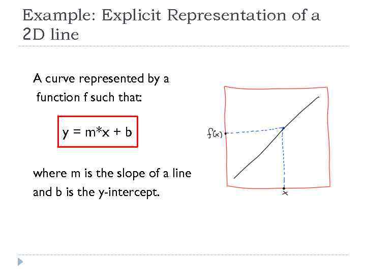Example: Explicit Representation of a 2 D line A curve represented by a function f such that: y = m*x + b where m is the slope of a line and b is the y-intercept.

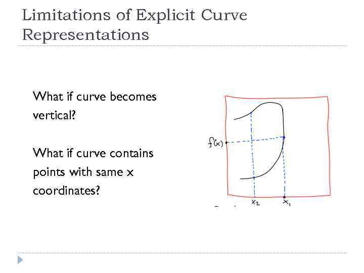Limitations of Explicit Curve Representations What if curve becomes vertical? What if curve contains points with same x coordinates?

Topic 1. 2 D Curve representations Explicit representation Parametric representation Tangent & normal vectors Implicit representation

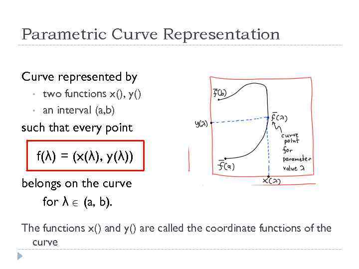Parametric Curve Representation Curve represented by • • two functions x(), y() an interval (a, b) such that every point f(λ) = (x(λ), y(λ)) belongs on the curve for λ (a, b). The functions x() and y() are called the coordinate functions of the curve

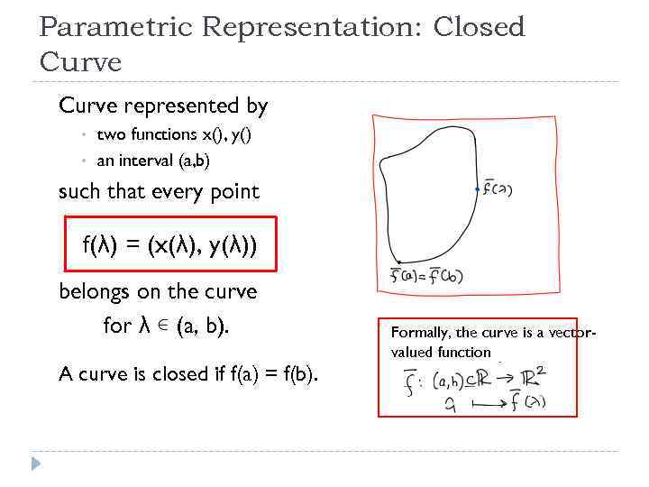Parametric Representation: Closed Curve represented by • • two functions x(), y() an interval (a, b) such that every point f(λ) = (x(λ), y(λ)) belongs on the curve for λ (a, b). A curve is closed if f(a) = f(b). Formally, the curve is a vectorvalued function

Parametric Representation: Smooth Curves Simple geometric objects (lines, circles, ellipses, etc) can be represented much more compactly using analytic expressions for x() and y() A curve is smooth if x(), y() have continuous derivatives

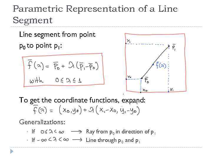Parametric Representation of a Line Segment Line segment from point p 0 to point p 1: To get the coordinate functions, expand: Generalizations: • • If If Ray from p 0 in direction of p 1 Line through p 0 and p 1

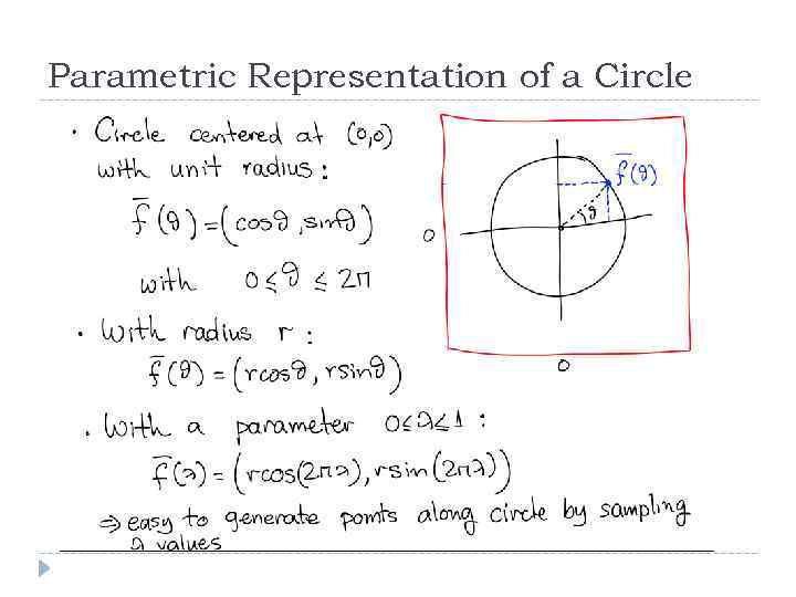Parametric Representation of a Circle

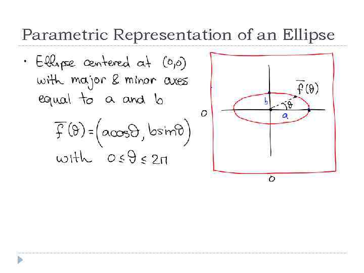Parametric Representation of an Ellipse

Topic 1. 2 D Curve representations Explicit representation Parametric representation Tangent & normal vectors Implicit representation

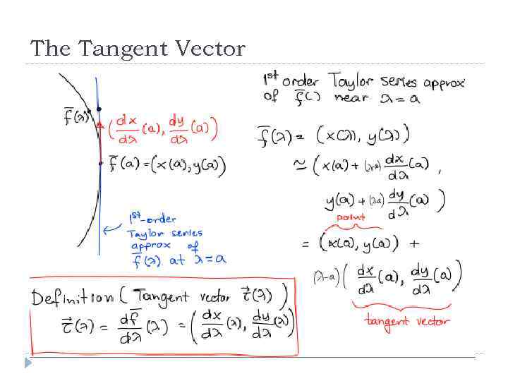The Tangent Vector

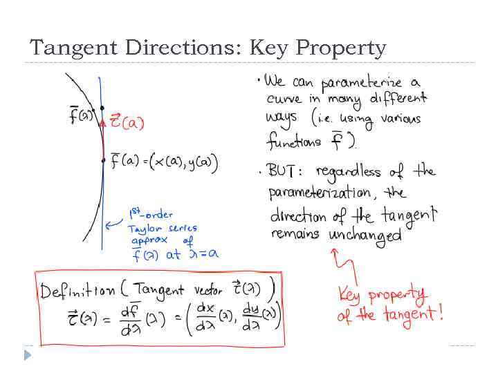Tangent Directions: Key Property

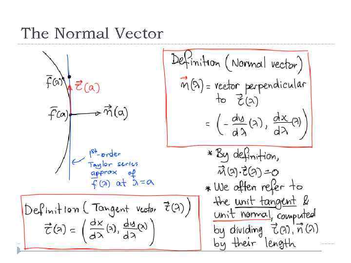The Normal Vector

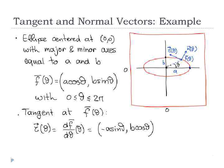Tangent and Normal Vectors: Example

Topic 1. 2 D Curve representations Explicit representation Parametric representation Tangent & normal vectors Implicit representation

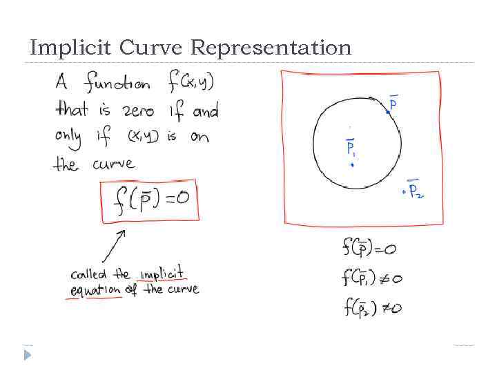Implicit Curve Representation

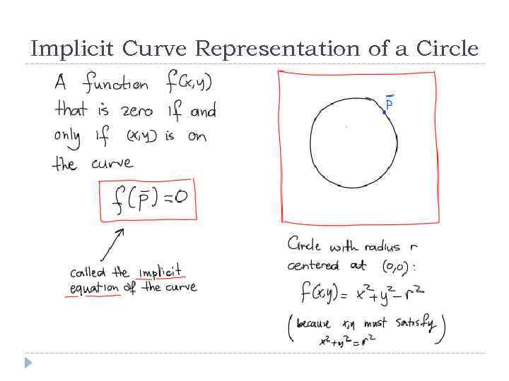Implicit Curve Representation of a Circle

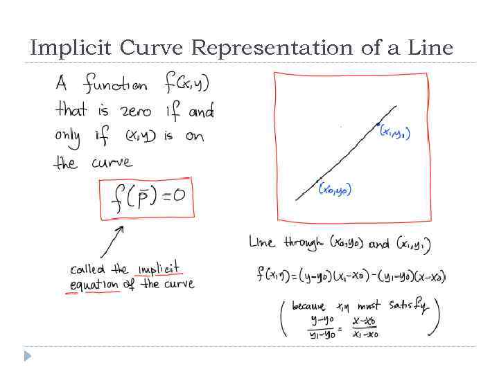Implicit Curve Representation of a Line

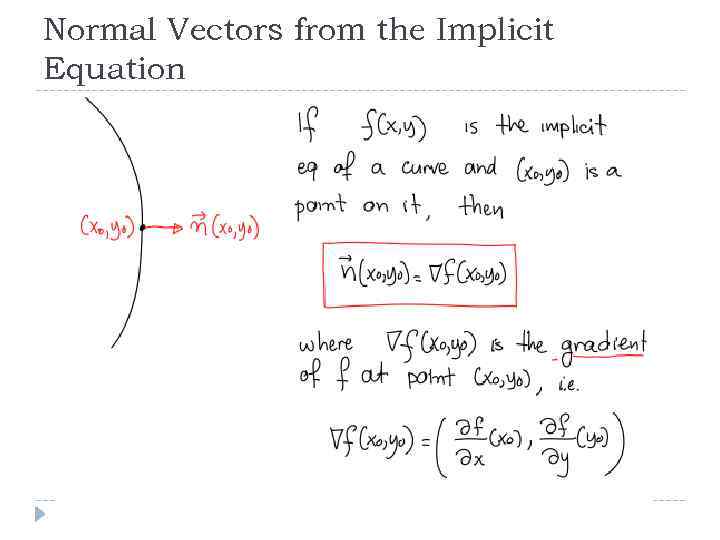Normal Vectors from the Implicit Equation

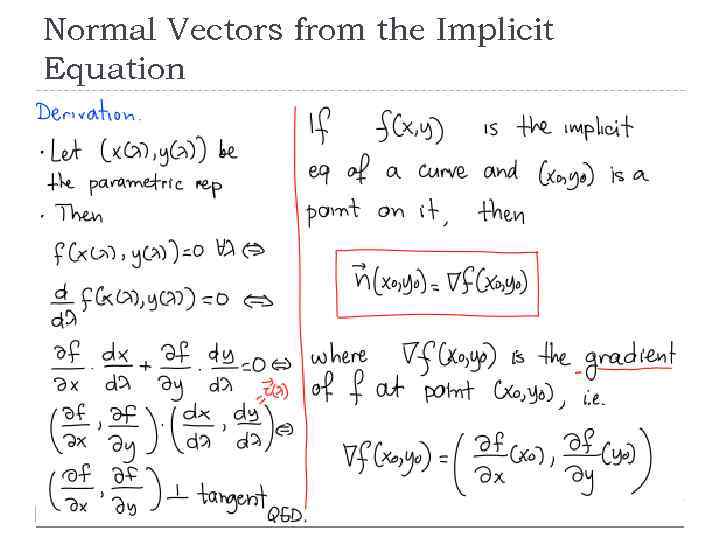Normal Vectors from the Implicit Equation