Computer Graphics 2 D Transformations Downloaded from http

Computer Graphics 2 D Transformations Downloaded from http: //www. comp. dit. ie/bmacnamee

2 of 45 Contents In today’s lecture we’ll cover the following: – Why transformations – Transformations • Translation • Scaling • Rotation – Homogeneous coordinates – Matrix multiplications – Combining transformations

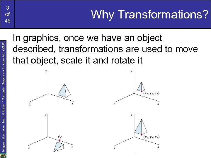Images taken from Hearn & Baker, “Computer Graphics with Open. GL” (2004) 3 of 45 Why Transformations? In graphics, once we have an object described, transformations are used to move that object, scale it and rotate it

6 of 45 Transformations Whole collections of points may be transformed by the same transformation T, e. g. lines or circles P 1 {0, 2} The image of a line, L, under T, is the set of all images of the individual points of L. For most mappings of interest, this image is still a connected curve of some shape For some mappings, the result of transforming a line may no longer be a line P 0 {0, 0} Q 1 {0, 4} P 2 {2, 2} P 3 {2, 0} Q 2 {4, 4} Affine Transformations, however, do preserve lines, and are the most commonly-used transformations in computer graphics Q 0 {0, 0} Q 3 {4, 0}

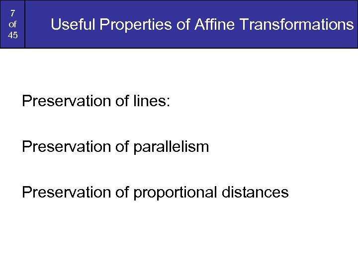7 of 45 Useful Properties of Affine Transformations Preservation of lines: Preservation of parallelism Preservation of proportional distances

8 of 45 Why are they useful? They preserve lines, so the image of a straight line is another straight line. This vastly simplifies drawing transformed line segments. We need only compute the image of the two endpoints of the original line and then draw a straight line between them Preservation of co-linearity guarantees that polygons will transform into polygons Preservation of parallelism guarantees that parallelograms will transform into parallelograms Preservation of proportional distances means that mid-points of lines remain mid-points

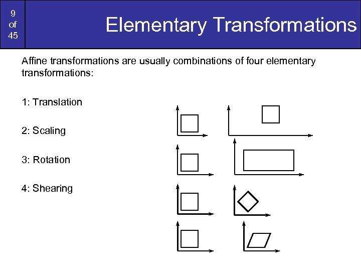9 of 45 Elementary Transformations Affine transformations are usually combinations of four elementary transformations: 1: Translation 2: Scaling 3: Rotation 4: Shearing

10 of 45 Translation Simply moves an object from one position to another xnew = xold + tx y ynew = yold + ty (tx, ty) is the translation vector or shift vector 6 5 4 3 2 1 0 1 2 3 4 5 6 7 8 9 10 Note: House shifts position relative to origin x

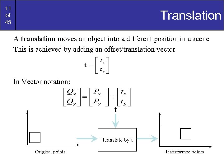11 of 45 Translation A translation moves an object into a different position in a scene This is achieved by adding an offset/translation vector In Vector notation: t Translate by t Original points Transformed points

12 of 45 Translation P/ = P + T

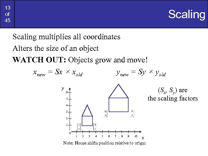13 of 45 Scaling multiplies all coordinates Alters the size of an object WATCH OUT: Objects grow and move! xnew = Sx × xold ynew = Sy × yold y (Sx, Sy) are the scaling factors 6 5 4 3 2 1 0 1 2 3 4 5 6 7 8 9 10 x Note: House shifts position relative to origin

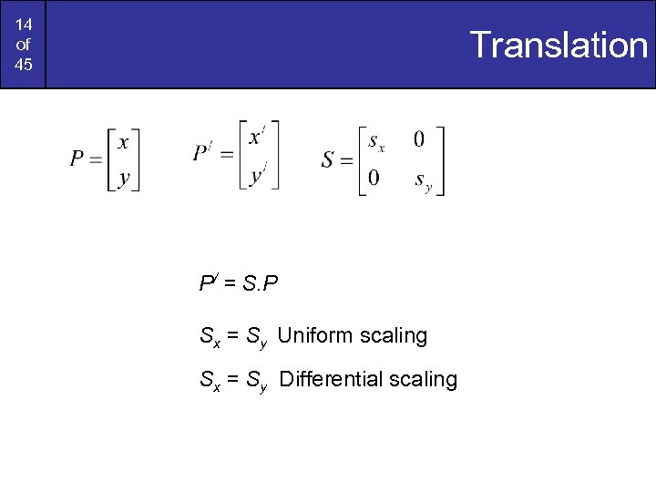14 of 45 Translation P/ = S. P Sx = Sy Uniform scaling Sx = Sy Differential scaling

15 of 45 Scaling A scaling changes the size of an object with two scale factors, Sx and Sy (if Sx != Sy, then we have a non-uniform scale) Sx, Sy Scale by Sx, Sy Original points Transformed points

16 of 45 Fixed Point Scaling • The location of a scaled object can be controlled by choosing a position, called the fixed point, (xf, yf) i. e. , to remain unchanged after the scaling transformation. • The fixed point can be chosen as the objects’ centroid or any other position • For a vertex with coordinates (x, y), the scaled coordinates (x/, y/) are calculated as, x/= xf + (x – xf)sx y/= yf + (y – yf)sy Þx/= x. sx + xf (1 – sx) and y/= y. sy + yf (1 – sy) Where xf (1 – sx) and yf (1 – sy) are constants for all points in the object.

17 of 45 Rotation To generate a rotation, a rotation angle θ and the position (xr, yr ) of the rotation point is needed xnew = r × cos(δ + θ) = r cosδ cosθ – r sin δ sinθ ynew = r × sin(δ + θ) = r cosδ sinθ + r sin δ cosθ Original polar coordinates xold = r cos δ and yold = r sin δ y 6 5 4 3 2 1 0 δ 1 2 3 4 5 6 7 8 9 10 x

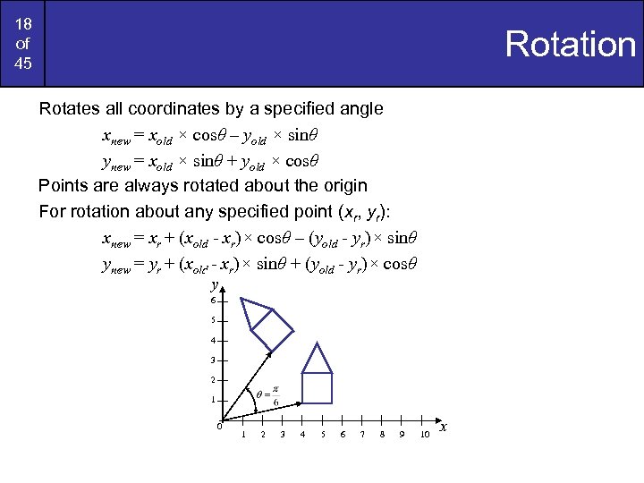18 of 45 Rotation Rotates all coordinates by a specified angle xnew = xold × cosθ – yold × sinθ ynew = xold × sinθ + yold × cosθ Points are always rotated about the origin For rotation about any specified point (xr, yr): xnew = xr + (xold - xr)× cosθ – (yold - yr)× sinθ ynew = yr + (xold - xr)× sinθ + (yold - yr)× cosθ y 6 5 4 3 2 1 0 1 2 3 4 5 6 7 8 9 10 x

19 of 45 Rotation equations can be written in the matrix form as P/ = R. P Where rotation matrix When coordinate positions are represented as row vectors instead of column vectors, the matrix product in rotation eqn (i) is transposed so that the trnsformed row coordinate [x’ y’] is calculated as P/ T = (R. P)T = PT. RT Where PT = [ x y ], and the transpose matrix RT of matrix R is obtained by interchanging rows & columns.

20 of 45 Rotation Using the trigonometric relations, a point rotated by an angle q about the origin is given by the following equations: So q Rotate by q Original points Transformed points

21 of 45 Rotation - derivation [1] [2] [3] [4] Q P PY R PX [1] Substituting from [3] and [4]… Similarly from [2]… Background info

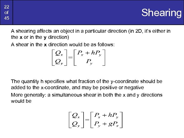22 of 45 Shearing A shearing affects an object in a particular direction (in 2 D, it’s either in the x or in the y direction) A shear in the x direction would be as follows: The quantity h specifies what fraction of the y-coordinate should be added to the x-coordinate, and may be positive or negative More generally: a simultaneous shear in both the x and y directions would be

23 of 45 Shearing g =0, h=0. 5 Shear by {g, h} Original points Transformed points g=0. 5, h=0. 5 Shear by {g, h} Original points Transformed points

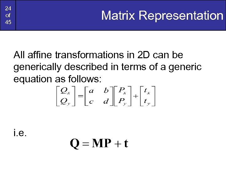24 of 45 Matrix Representation All affine transformations in 2 D can be generically described in terms of a generic equation as follows: i. e.

25 of 45 Transformations Summary n 1: Translation n 2: Scaling T n 3: Rotation T n 4: Shearing T T

26 of 45 Problem An affine transformation is composed of a linear combination followed by a translation Unfortunately, the translation portion is not a matrix multiplication but must instead be added as an extra term, or vector – this is inconvenient

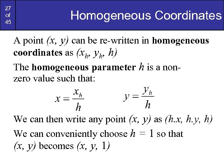27 of 45 Homogeneous Coordinates A point (x, y) can be re-written in homogeneous coordinates as (xh, yh, h) The homogeneous parameter h is a nonzero value such that: We can then write any point (x, y) as (h. x, h. y, h) We can conveniently choose h = 1 so that (x, y) becomes (x, y, 1)

28 of 45 Why Homogeneous Coordinates? Mathematicians commonly use homogeneous coordinates as they allow scaling factors to be removed from equations We will see in a moment that all of the transformations we discussed previously can be represented as 3*3 matrices Using homogeneous coordinates allows us use matrix multiplication to calculate transformations – extremely efficient!

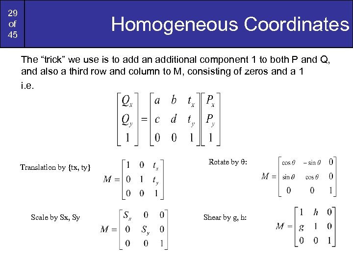29 of 45 Homogeneous Coordinates The “trick” we use is to add an additional component 1 to both P and Q, and also a third row and column to M, consisting of zeros and a 1 i. e. Translation by {tx, ty} Scale by Sx, Sy Rotate by q: Shear by g, h:

30 of 45 Homogeneous Translation The translation of a point by (dx, dy) can be written in matrix form as: Representing the point as a homogeneous column vector we perform the calculation as:

31 of 45 Remember Matrix Multiplication Recall how matrix multiplication takes place:

32 of 45 Homogenous Coordinates To make operations easier, 2 -D points are written as homogenous coordinate column vectors Translation: Scaling:

33 of 45 Homogenous Coordinates (cont…) Rotation:

34 of 45 Inverse Transformations can easily be reversed using inverse transformations

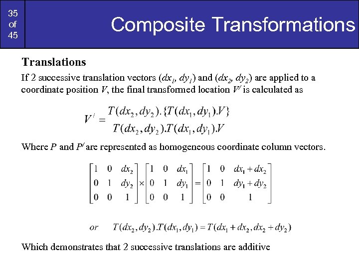35 of 45 Composite Transformations Translations If 2 successive translation vectors (dx 1, dy 1) and (dx 2, dy 2) are applied to a coordinate position V, the final transformed location V/ is calculated as Where P and P/ are represented as homogeneous coordinate column vectors. Which demonstrates that 2 successive translations are additive

36 of 45 Composite Transformations Rotations If 2 successive rotation vectors are applied to a coordinate position V, the final rotated location V/ is calculated as By multiplying the 2 rotation matrices, we can verify that 2 scuccessive rotations are additive: . So that the final rotated coordinates can be calculated with the composite matrix as

37 of 45 Composite Transformations Scalings Concatenating transformation matrices for 2 successive scaling operations produces the following composite scaling matrix: Which demonstrates that 2 successive scalings are multiplicative. Thus if we were to triple the size of an object twice in succession, the final size would be nine times that of the original.

38 of 45 Combining Transformations A number of transformations can be combined into one matrix to make things easy – Allowed by the fact that we use homogenous coordinates Imagine rotating a polygon around a point other than the origin – Transform to centre point to origin – Rotate around origin – Transform back to centre point

39 of 45 Combining Transformations (cont…) 2 1 3 4

40 of 45 Combining Transformations (cont…) The three transformation matrices are combined as follows REMEMBER: Matrix multiplication is not commutative so order matters

41 of 45 Summary In this lecture we have taken a look at: – 2 D Transformations • Translation • Scaling • Rotation – Homogeneous coordinates – Matrix multiplications – Combining transformations Next time we’ll start to look at how we take these abstract shapes etc and get them onscreen

42 of 45 Exercises 1 Translate the shape below by (7, 2) y 6 5 4 (2, 3) 3 (1, 2) 2 (3, 2) 1 (2, 1) 0 1 2 3 4 5 6 7 8 9 10 x

43 of 45 Exercises 2 Scale the shape below by 3 in x and 2 in y y 6 5 4 (2, 3) 3 (1, 2) 2 (3, 2) 1 (2, 1) 0 1 2 3 4 5 6 7 8 9 10 x

44 of 45 Exercises 3 Rotate the shape below by 30° about the origin y 6 5 4 (7, 3) 3 (6, 2) 2 (8, 2) 1 (7, 1) 0 1 2 3 4 5 6 7 8 9 10 x

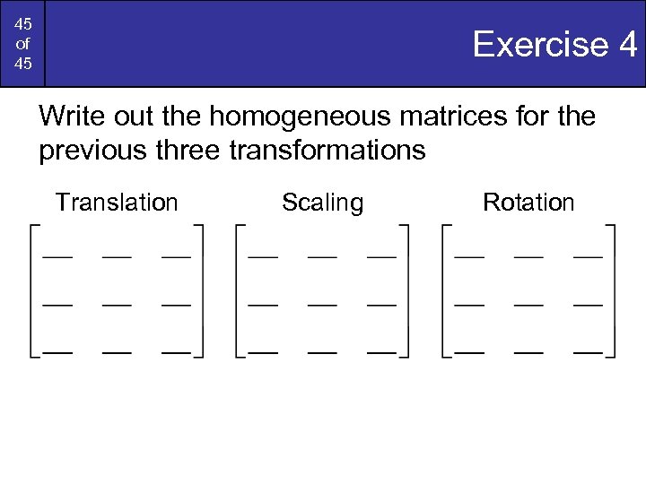45 of 45 Exercise 4 Write out the homogeneous matrices for the previous three transformations Translation Scaling Rotation

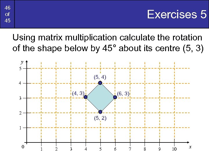46 of 45 Exercises 5 Using matrix multiplication calculate the rotation of the shape below by 45° about its centre (5, 3) y 5 (5, 4) 4 (4, 3) 3 (6, 3) 2 (5, 2) 1 0 1 2 3 4 5 6 7 8 9 10 x

47 of 45 Scratch y 6 5 4 3 2 1 0 1 2 3 4 5 6 7 8 9 10 x

48 of 45 Equations Translation: xnew = xold + dx ynew = yold + dy Scaling: xnew = Sx × xold ynew = Sy × yold Rotation xnew = xold × cosθ – yold × sinθ ynew = xold × sinθ + yold × cosθ