Computational Rules DATA USED IN ECONOMETRICS CROSS-SECTION

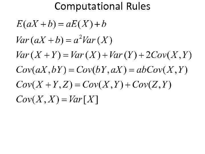Computational Rules

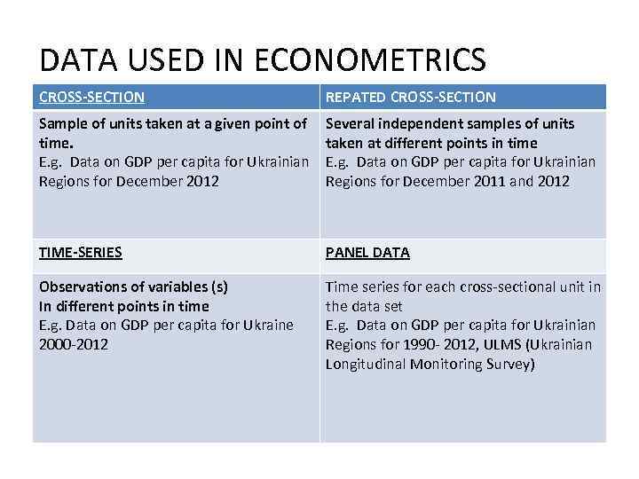DATA USED IN ECONOMETRICS CROSS-SECTION REPATED CROSS-SECTION Sample of units taken at a given point of time. E. g. Data on GDP per capita for Ukrainian Regions for December 2012 Several independent samples of units taken at different points in time E. g. Data on GDP per capita for Ukrainian Regions for December 2011 and 2012 TIME-SERIES PANEL DATA Observations of variables (s) In different points in time E. g. Data on GDP per capita for Ukraine 2000 -2012 Time series for each cross-sectional unit in the data set E. g. Data on GDP per capita for Ukrainian Regions for 1990 - 2012, ULMS (Ukrainian Longitudinal Monitoring Survey)

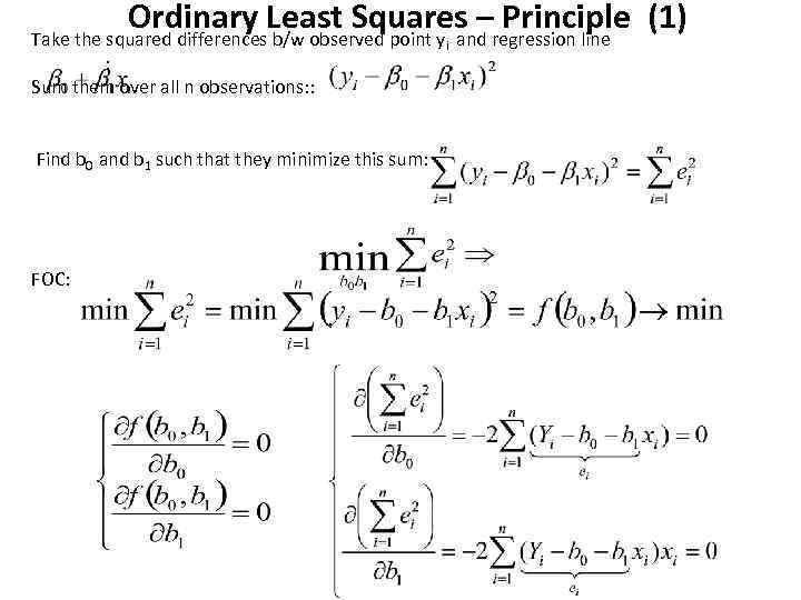Ordinary Least Squares –regression line (1) Principle Take the squared differences b/w observed point y and : Sum them over all n observations: : Find b 0 and b 1 such that they minimize this sum: FOC: i

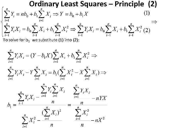Ordinary Least Squares – Principle (2) To solve for b 1 we substitute (1) into (2):

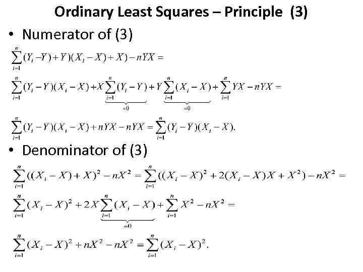Ordinary Least Squares – Principle (3) • Numerator of (3) • Denominator of (3)

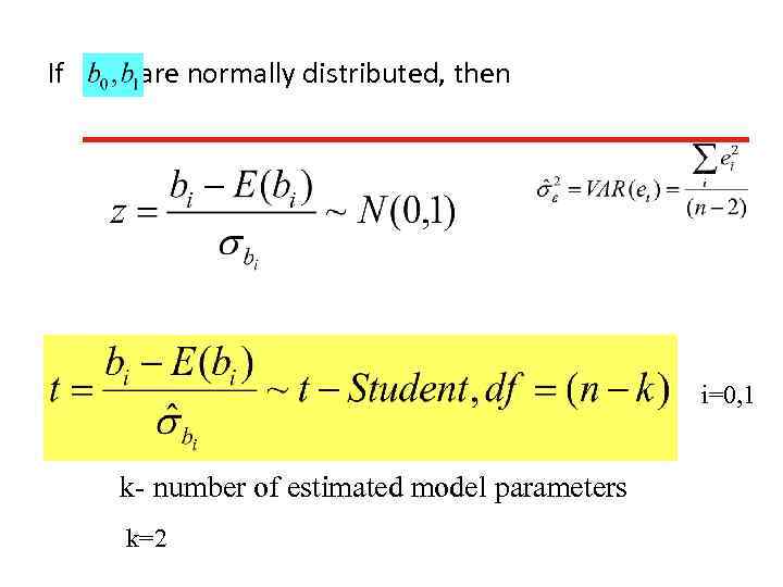If are normally distributed, then i=0, 1. k- number of estimated model parameters k=2

.

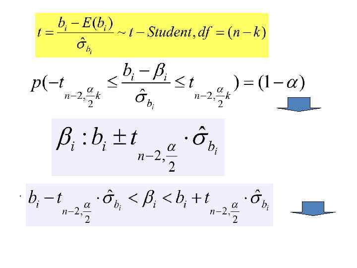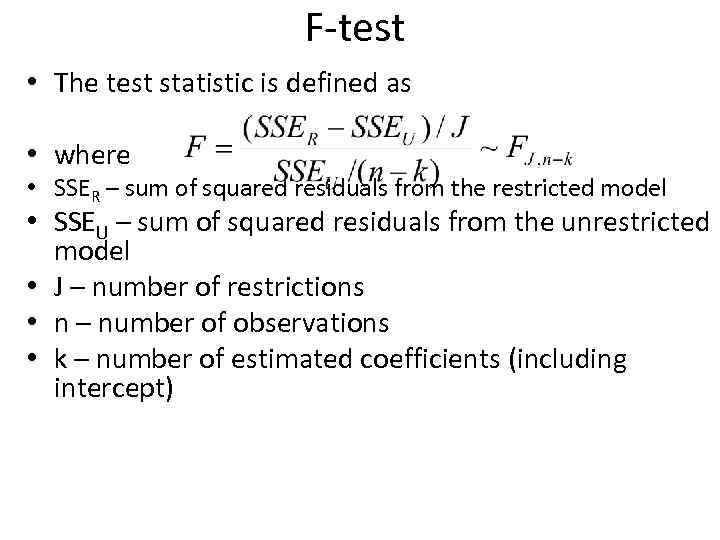F-test • The test statistic is defined as • where • SSER – sum of squared residuals from the restricted model • SSEU – sum of squared residuals from the unrestricted model • J – number of restrictions • n – number of observations • k – number of estimated coefficients (including intercept)

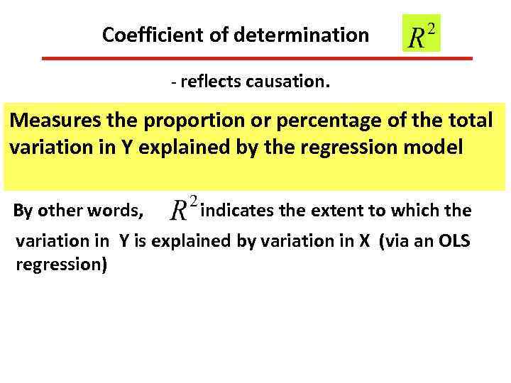Coefficient of determination - reflects causation. Measures the proportion or percentage of the total variation in Y explained by the regression model By other words, indicates the extent to which the variation in Y is explained by variation in X (via an OLS regression)

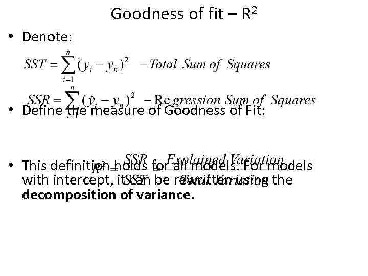Goodness of fit – R 2 • Denote: • Define the measure of Goodness of Fit: • This definition holds for all models. For models with intercept, it can be rewritten using the decomposition of variance.

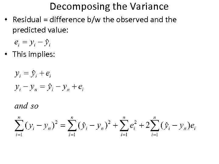Decomposing the Variance • Residual = difference b/w the observed and the predicted value: • This implies:

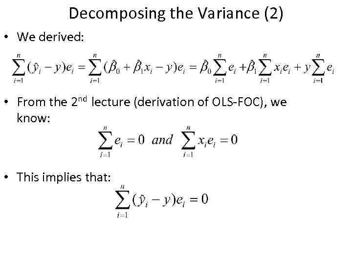Decomposing the Variance (2) • We derived: • From the 2 nd lecture (derivation of OLS-FOC), we know: • This implies that:

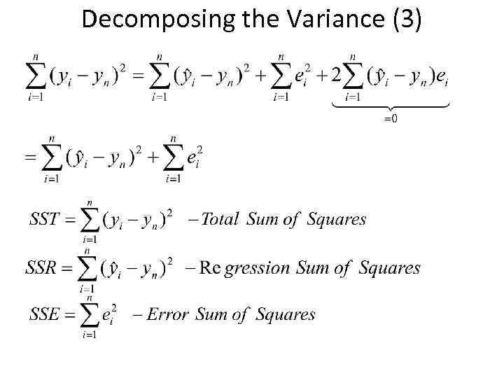Decomposing the Variance (3)

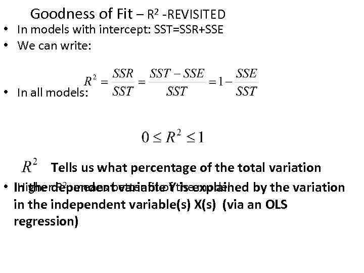Goodness of Fit – R 2 -REVISITED • In models with intercept: SST=SSR+SSE • We can write: • In all models: Tells us what percentage of the total variation • In the dependent variable Ytheexplained by the variation Higher R 2 means better fit of is model in the independent variable(s) X(s) (via an OLS regression)

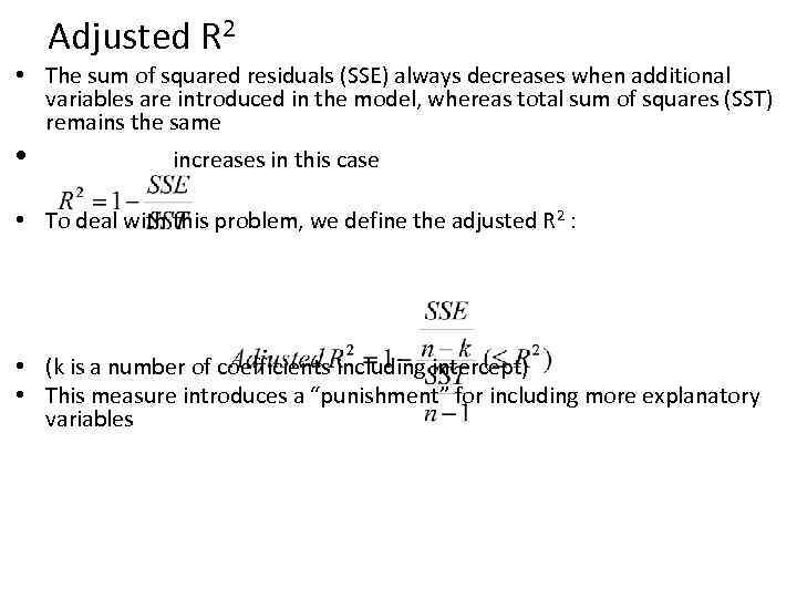Adjusted R 2 • The sum of squared residuals (SSE) always decreases when additional variables are introduced in the model, whereas total sum of squares (SST) remains the same • increases in this case • To deal with this problem, we define the adjusted R 2 : • (k is a number of coefficients including intercept) • This measure introduces a “punishment” for including more explanatory variables

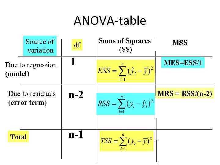АNOVA-table Source of variation Due to regression (model) df 1 Due to residuals (error term) n-2 Total n-1 Sums of Squares (SS) MSS MES=ESS/1 MRS = RSS/(n-2)

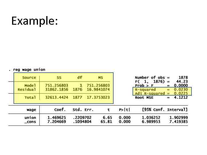Example:

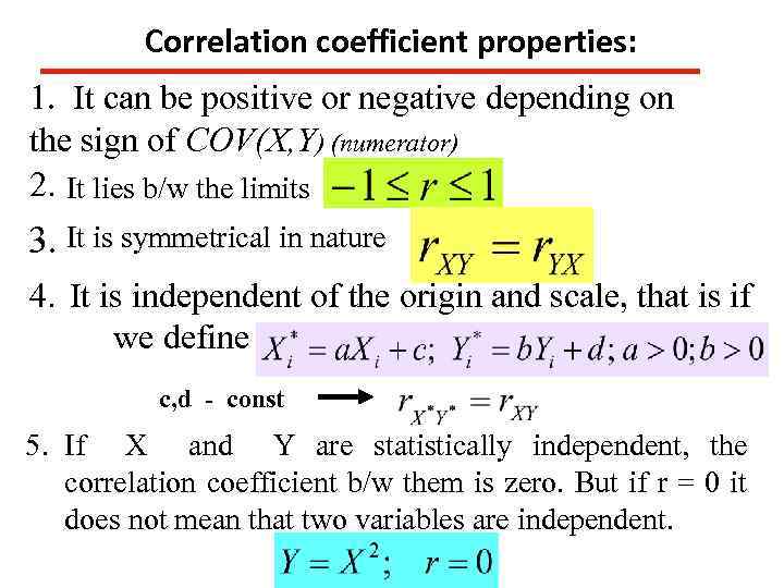Correlation coefficient properties: 1. It can be positive or negative depending on the sign of COV(X, Y) (numerator) 2. It lies b/w the limits 3. It is symmetrical in nature 4. It is independent of the origin and scale, that is if we define c, d - const 5. If Х and Y are statistically independent, the correlation coefficient b/w them is zero. But if r = 0 it does not mean that two variables are independent.

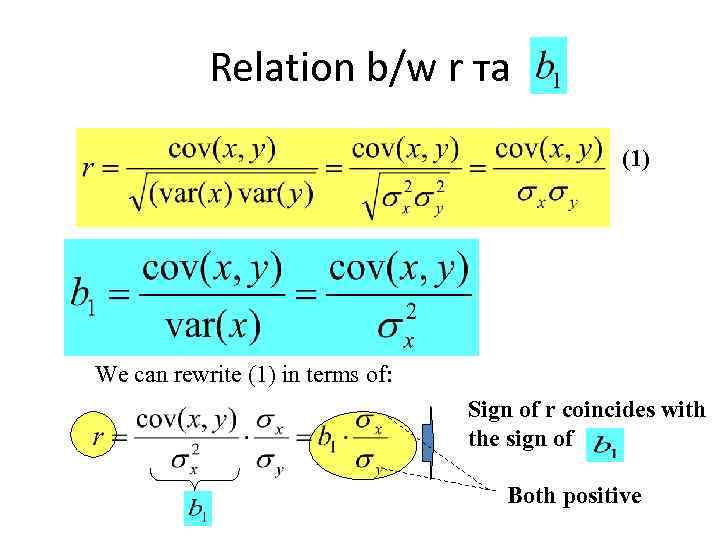Relation b/w r та (1) We can rewrite (1) in terms of: Sign of r coincides with the sign of Both positive

Relation b/w r та We can rewrite