Computational Neuroanatomy John Ashburner john fil ion ucl ac

Computational Neuroanatomy John Ashburner john@fil. ion. ucl. ac. uk z z z Smoothing Rigid registration Spatial normalisation Segmentation Morphometry

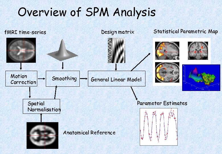
Overview of SPM Analysis Motion Correction Statistical Parametric Map Design matrix f. MRI time-series Smoothing General Linear Model Parameter Estimates Spatial Normalisation Anatomical Reference

Contents z. Smoothing z. Rigid Registration z. Spatial normalisation z. Segmentation z. Morphometry

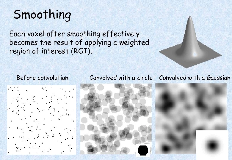
Smoothing Each voxel after smoothing effectively becomes the result of applying a weighted region of interest (ROI). Before convolution Convolved with a circle Convolved with a Gaussian

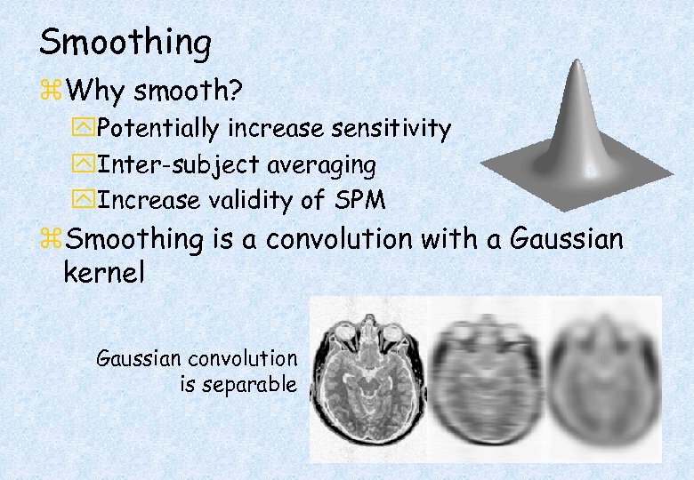
Smoothing z. Why smooth? y. Potentially increase sensitivity y. Inter-subject averaging y. Increase validity of SPM z. Smoothing is a convolution with a Gaussian kernel Gaussian convolution is separable

Contents z. Smoothing z. Rigid Registration y. Rigid-body transforms y. Optimisation & objective functions y. Interpolation z. Spatial normalisation z. Segmentation z. Morphometry

Within-subject Registration z. Assumes there is no shape change, and motion is rigid-body z. Used by [Realign] and [Coregister] functions z. The steps are: z. Registration - i. e. Optimising the parameters that describe a rigid body transformation between the source and reference images z. Transformation - i. e. Re-sampling according to the determined transformation

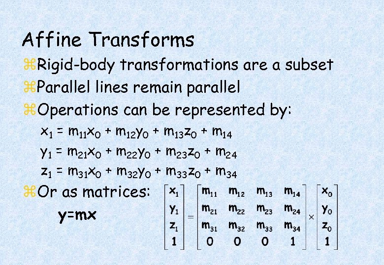
Affine Transforms z. Rigid-body transformations are a subset z. Parallel lines remain parallel z. Operations can be represented by: x 1 = m 11 x 0 + m 12 y 0 + m 13 z 0 + m 14 y 1 = m 21 x 0 + m 22 y 0 + m 23 z 0 + m 24 z 1 = m 31 x 0 + m 32 y 0 + m 33 z 0 + m 34 z. Or as matrices: y=mx

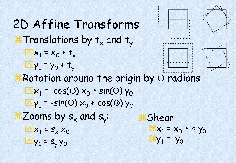
2 D Affine Transforms z. Translations by tx and ty yx 1 = x 0 + t x yy 1 = y 0 + t y z. Rotation around the origin by radians yx 1 = cos( ) x 0 + sin( ) y 0 yy 1 = -sin( ) x 0 + cos( ) y 0 z. Zooms by sx and sy: yx 1 = s x x 0 yy 1 = s y y 0 z. Shear zx 1 = x 0 + h y 0 zy 1 = y 0

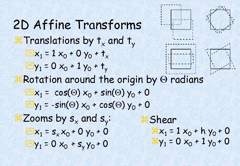
2 D Affine Transforms z. Translations by tx and ty yx 1 = 1 x 0 + 0 y 0 + t x yy 1 = 0 x 0 + 1 y 0 + t y z. Rotation around the origin by radians yx 1 = cos( ) x 0 + sin( ) y 0 + 0 yy 1 = -sin( ) x 0 + cos( ) y 0 + 0 z. Zooms by sx and sy: yx 1 = s x x 0 + 0 yy 1 = 0 x 0 + s y y 0 + 0 z. Shear zx 1 = 1 x 0 + h y 0 + 0 zy 1 = 0 x 0 + 1 y 0 + 0

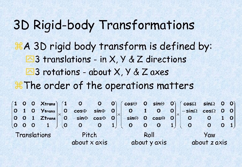
3 D Rigid-body Transformations z. A 3 D rigid body transform is defined by: y 3 translations - in X, Y & Z directions y 3 rotations - about X, Y & Z axes z. The order of the operations matters Translations Pitch about x axis Roll about y axis Yaw about z axis

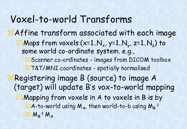
Voxel-to-world Transforms z. Affine transform associated with each image y. Maps from voxels (x=1. . Nx, y=1. . Ny, z=1. . Nz) to some world co-ordinate system. e. g. , x. Scanner co-ordinates - images from DICOM toolbox x. T&T/MNI coordinates - spatially normalised z. Registering image B (source) to image A (target) will update B’s vox-to-world mapping y. Mapping from voxels in A to voxels in B is by x. A-to-world using MA, then world-to-b using MB-1 x MB-1 MA

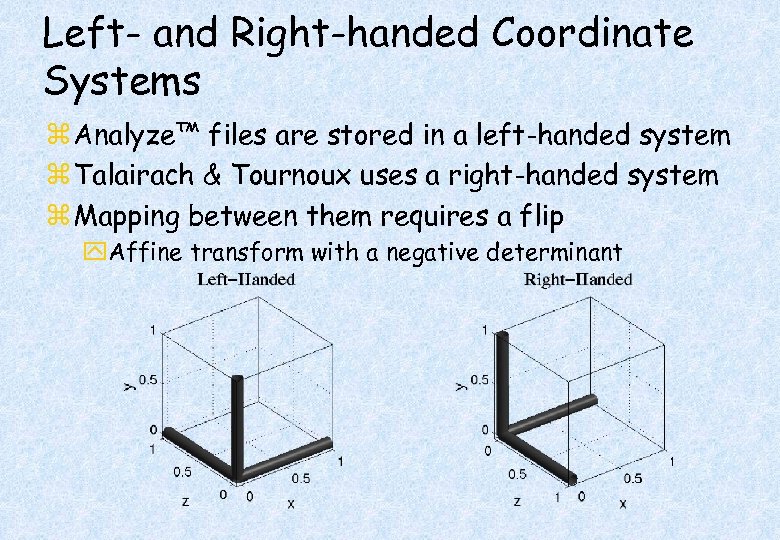
Left- and Right-handed Coordinate Systems z Analyze™ files are stored in a left-handed system z Talairach & Tournoux uses a right-handed system z Mapping between them requires a flip y. Affine transform with a negative determinant

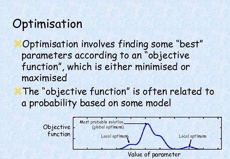
Optimisation z. Optimisation involves finding some “best” parameters according to an “objective function”, which is either minimised or maximised z. The “objective function” is often related to a probability based on some model Objective function Most probable solution (global optimum) Local optimum Value of parameter

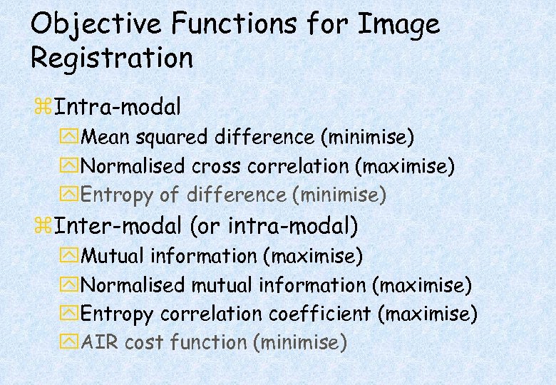
Objective Functions for Image Registration z. Intra-modal y. Mean squared difference (minimise) y. Normalised cross correlation (maximise) y. Entropy of difference (minimise) z. Inter-modal (or intra-modal) y. Mutual information (maximise) y. Normalised mutual information (maximise) y. Entropy correlation coefficient (maximise) y. AIR cost function (minimise)

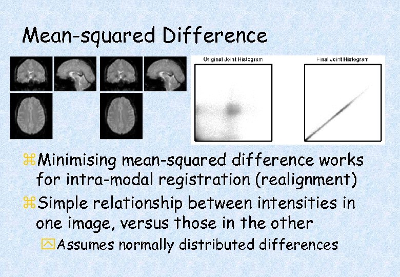
Mean-squared Difference z. Minimising mean-squared difference works for intra-modal registration (realignment) z. Simple relationship between intensities in one image, versus those in the other y. Assumes normally distributed differences

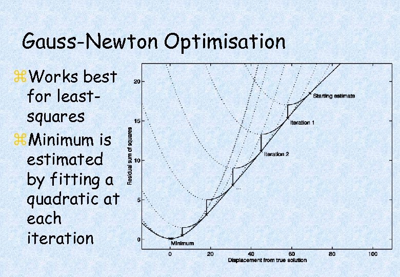
Gauss-Newton Optimisation z. Works best for leastsquares z. Minimum is estimated by fitting a quadratic at each iteration

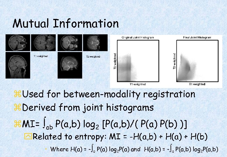
Mutual Information z. Used for between-modality registration z. Derived from joint histograms z. MI= ab P(a, b) log 2 [P(a, b)/( P(a) P(b) )] y. Related to entropy: MI = -H(a, b) + H(a) + H(b) • Where H(a) = - a P(a) log 2 P(a) and H(a, b) = - a P(a, b) log 2 P(a, b)

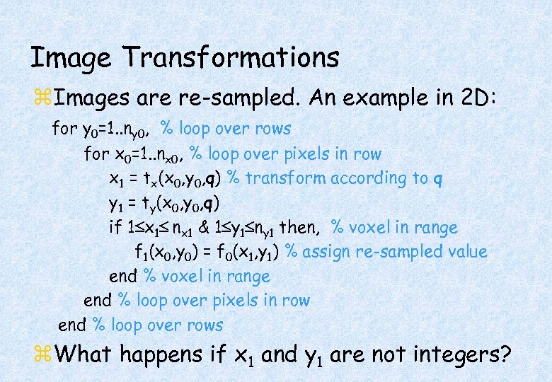
Image Transformations z. Images are re-sampled. An example in 2 D: for y 0=1. . ny 0, % loop over rows for x 0=1. . nx 0, % loop over pixels in row x 1 = tx(x 0, y 0, q) % transform according to q y 1 = ty(x 0, y 0, q) if 1 x 1 nx 1 & 1 y 1 ny 1 then, % voxel in range f 1(x 0, y 0) = f 0(x 1, y 1) % assign re-sampled value end % voxel in range end % loop over pixels in row end % loop over rows z. What happens if x 1 and y 1 are not integers?

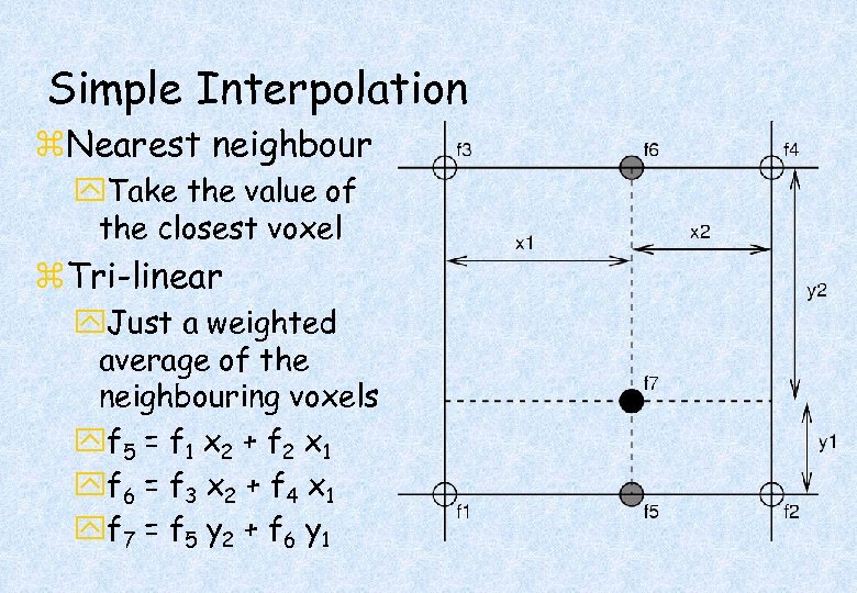
Simple Interpolation z. Nearest neighbour y. Take the value of the closest voxel z. Tri-linear y. Just a weighted average of the neighbouring voxels yf 5 = f 1 x 2 + f 2 x 1 yf 6 = f 3 x 2 + f 4 x 1 yf 7 = f 5 y 2 + f 6 y 1

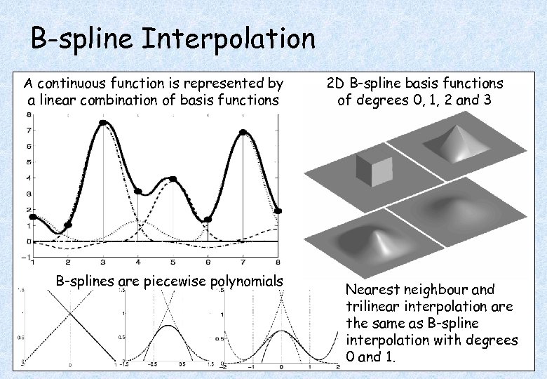
B-spline Interpolation A continuous function is represented by a linear combination of basis functions B-splines are piecewise polynomials 2 D B-spline basis functions of degrees 0, 1, 2 and 3 Nearest neighbour and trilinear interpolation are the same as B-spline interpolation with degrees 0 and 1.

Contents z. Smoothing z. Rigid Registration z. Spatial normalisation y. Affine registration y. Nonlinear registration y. Regularisation z. Segmentation z. Morphometry

Spatial Normalisation - Reasons z. Inter-subject averaging y. Increase sensitivity with more subjects xfixed-effects analysis y. Extrapolate findings to the population as a whole xmixed-effects analysis z. Standard coordinate system ye. g. Talairach & Tournoux space

Spatial Normalisation - Objective z. Warp the images such that functionally homologous regions from different subjects are as close together as possible y. Problems: x. No exact match between structure and function x. Different brains are organised differently x. Computational problems (local minima, not enough information in the images, computationally expensive) z. Compromise by correcting gross differences followed by smoothing of normalised images

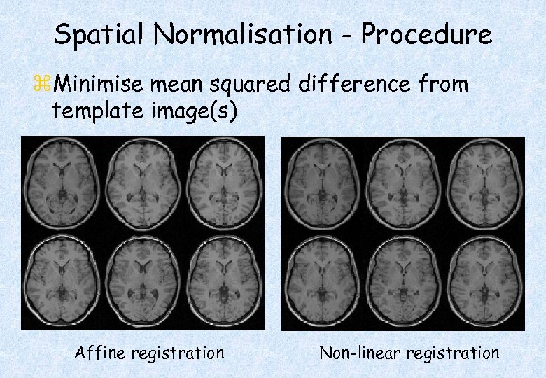
Spatial Normalisation - Procedure z. Minimise mean squared difference from template image(s) Affine registration Non-linear registration

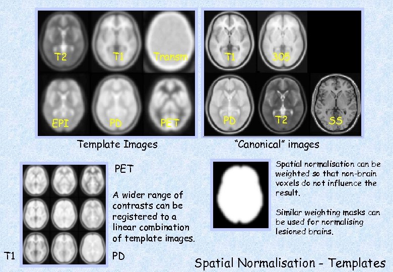
T 2 T 1 Transm T 1 305 EPI PD PET PD T 2 Template Images “Canonical” images PET A wider range of contrasts can be registered to a linear combination of template images. T 1 PD SS Spatial normalisation can be weighted so that non-brain voxels do not influence the result. Similar weighting masks can be used for normalising lesioned brains. Spatial Normalisation - Templates

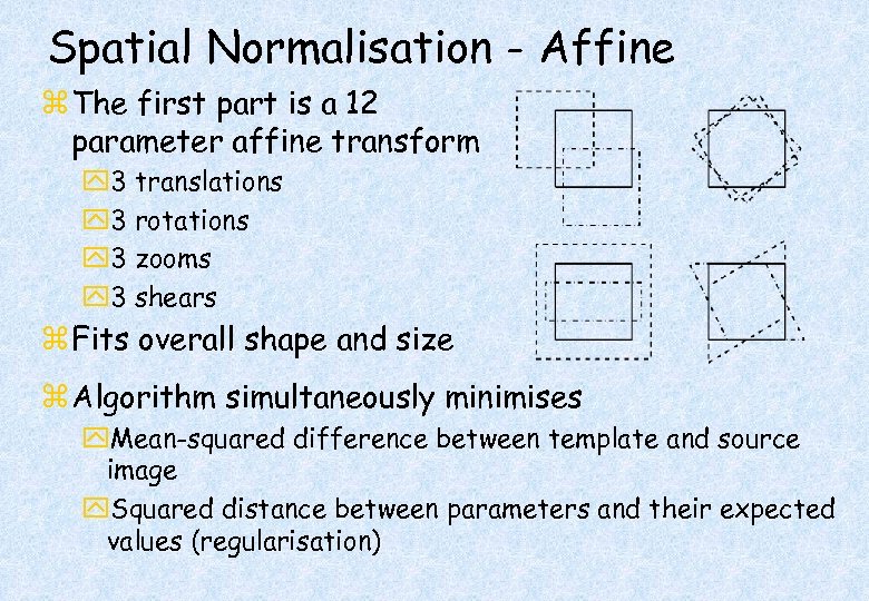
Spatial Normalisation - Affine z The first part is a 12 parameter affine transform y 3 translations y 3 rotations y 3 zooms y 3 shears z Fits overall shape and size z Algorithm simultaneously minimises y. Mean-squared difference between template and source image y. Squared distance between parameters and their expected values (regularisation)

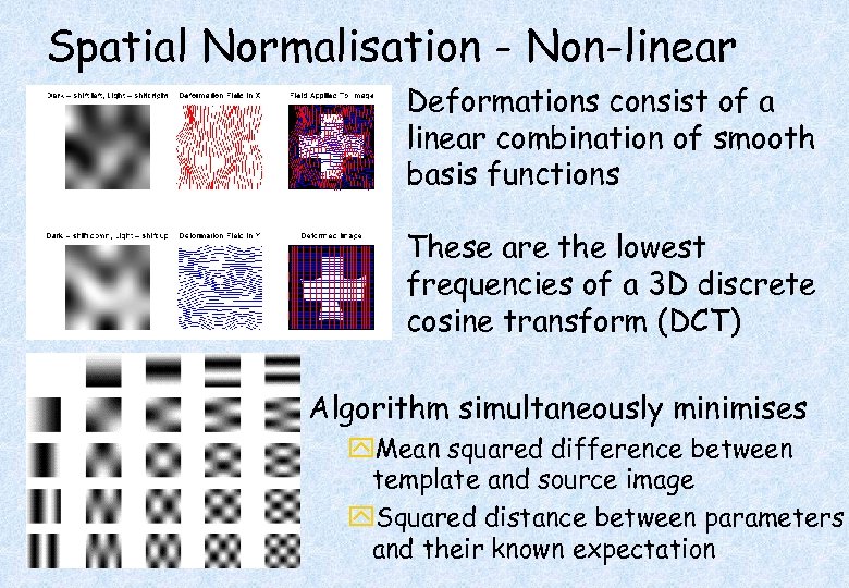
Spatial Normalisation - Non-linear Deformations consist of a linear combination of smooth basis functions These are the lowest frequencies of a 3 D discrete cosine transform (DCT) Algorithm simultaneously minimises y. Mean squared difference between template and source image y. Squared distance between parameters and their known expectation

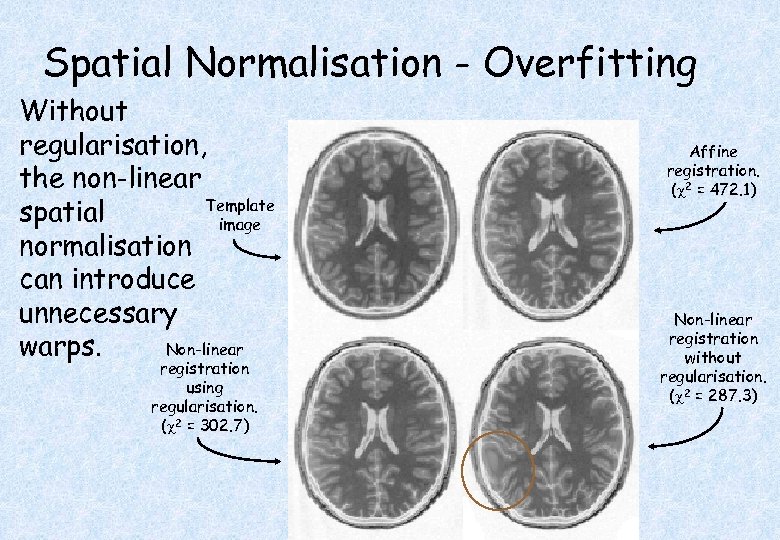
Spatial Normalisation - Overfitting Without regularisation, the non-linear Template spatial image normalisation can introduce unnecessary Non-linear warps. registration using regularisation. ( 2 = 302. 7) Affine registration. ( 2 = 472. 1) Non-linear registration without regularisation. ( 2 = 287. 3)

Contents z. Smoothing z. Rigid Registration z. Spatial normalisation z. Segmentation y. Gaussian mixture model y. Including prior probability maps y. Intensity non-uniformity correction z. Morphometry

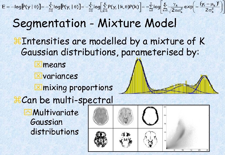
Segmentation - Mixture Model z. Intensities are modelled by a mixture of K Gaussian distributions, parameterised by: xmeans xvariances xmixing proportions z. Can be multi-spectral y. Multivariate Gaussian distributions

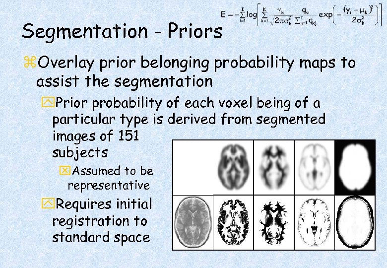
Segmentation - Priors z. Overlay prior belonging probability maps to assist the segmentation y. Prior probability of each voxel being of a particular type is derived from segmented images of 151 subjects x. Assumed to be representative y. Requires initial registration to standard space

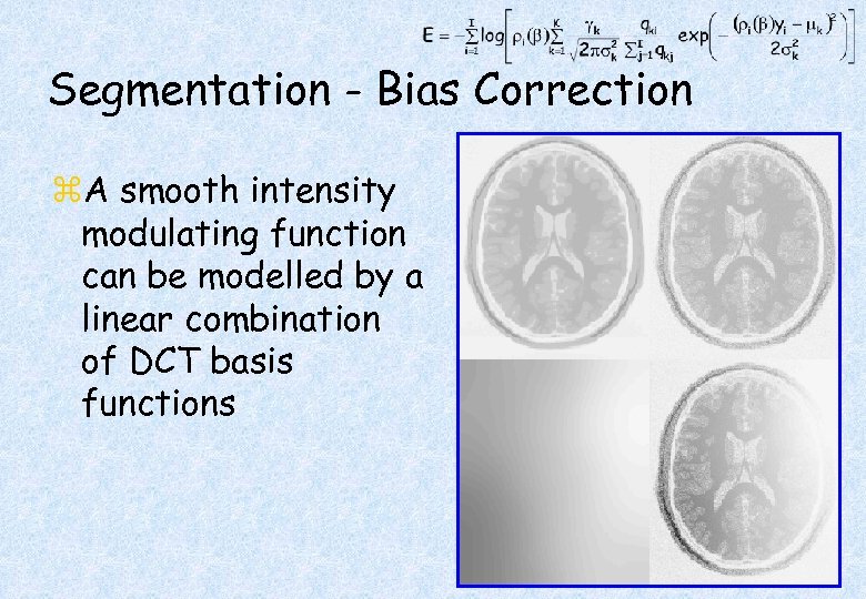
Segmentation - Bias Correction z. A smooth intensity modulating function can be modelled by a linear combination of DCT basis functions

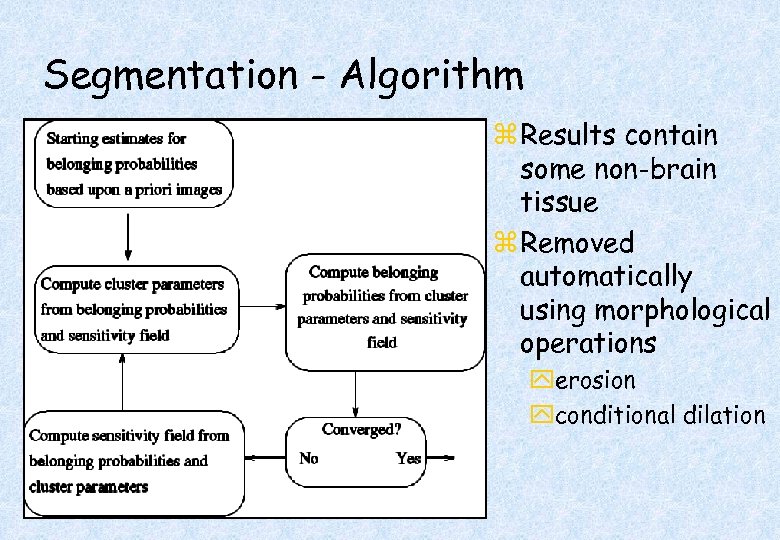
Segmentation - Algorithm z Results contain some non-brain tissue z Removed automatically using morphological operations yerosion yconditional dilation

Contents z. Smoothing z. Rigid Registration z. Spatial normalisation z. Segmentation z. Morphometry y. Volumes from deformations y. Voxel-based morphometry

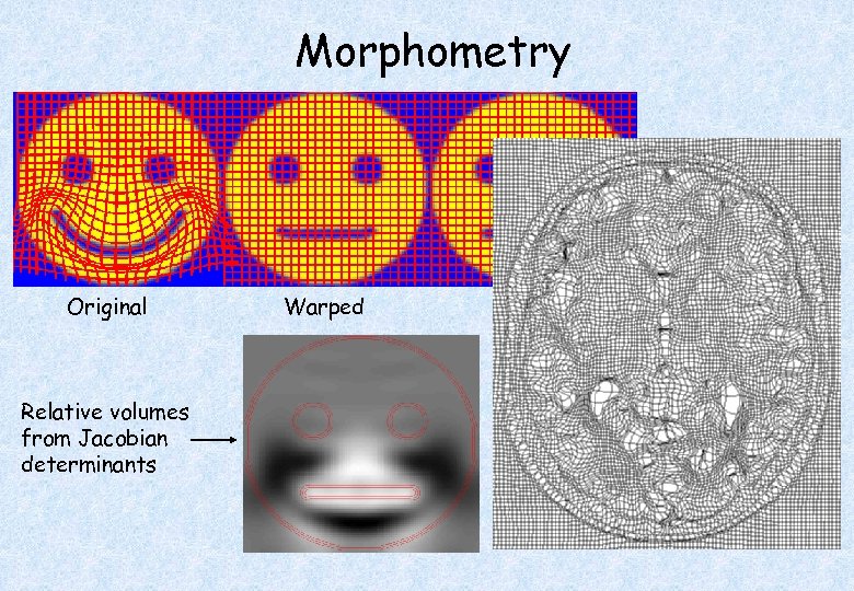
Morphometry Original Relative volumes from Jacobian determinants Warped Template

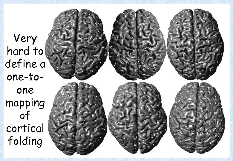
Very hard to define a one-toone mapping of cortical folding

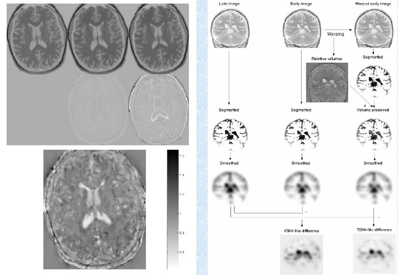
Early Late Difference Data from the Dementia Research Group, Queen Square.

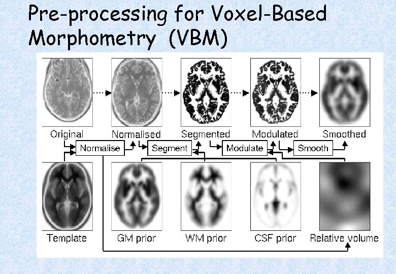
Pre-processing for Voxel-Based Morphometry (VBM)

References Friston et al (1995): Spatial registration and normalisation of images. Human Brain Mapping 3(3): 165 -189 Ashburner & Friston (1997): Multimodal image coregistration and partitioning - a unified framework. Neuro. Image 6(3): 209 -217 Collignon et al (1995): Automated multimodality image registration based on information theory. IPMI’ 95 pp 263 -274 Ashburner et al (1997): Incorporating prior knowledge into image registration. Neuro. Image 6(4): 344 -352 Ashburner et al (1999): Nonlinear spatial normalisation using basis functions. Human Brain Mapping 7(4): 254 -266 Ashburner & Friston (2000): Voxel-based morphometry - the methods. Neuro. Image 11: 805 -821