Computational Genomics Izabela Makalowska July 15 2006

Computational Genomics Izabela Makalowska July 15, 2006

The main task in modern biology is to find out how this… TGCATCGTAGCTAGCGCATGCTAGCTAGCTACGATGCATCGATGCTAGCTAGCATGCTAGCTATTGG CGCTAGCATGCATCGATGCATCGATTATAAGCGCGATGACGTCAG CGCGCGCATTATGCCGCGGCATGCTGCGCACAGTACTATAGCATTAGTAAAAA GGCCGCGTATATTTTACACGATAGTGCGGCGCGTAGCTAGTGCTAGTC TCCGGTTACACAGGTAGCTAGCTGCTAGCTGCTGCATGCATTAGT AGCTAGTGTAGCTAGCATGCTGCTAGCATGCATCGGGCGCGATGCT GCTAGCGCTGCTAGCTAGCTAGGCGCTAATTATTTTGGGGGGTTA AAAAATTTCGCTGCTTATACCCCCACATGATGATCGTTAGTAGCTACT AGCTCTCATCGCGCGGGGGGATGCTTAGCGTGGTGTGTGGTGTGGTC CTATAATTAGTGCATCGGCGCATCGATGGCTAGTCGATCGATTTTATATATCT AAAGACCCCATCTCTCTTTTCCCTTCTCTCGCTAGCGGTACGATTTACC

…becomes this

DNA sequence contains all information but we need to decipher it. TGCATCGTAGCTAGCGCATGCTAGCTAGCTACGATGCATCGATGCTAGCTAGCATGCTAGCTATTGG CGCTAGCATGCATCGATGCATCGATTATAAGCGCGATGACGTCAG CGCGCGCATTATGCCGCGGCATGCTGCGCACAGTACTATAGCATTAGTAAAAA GGCCGCGTATATTTTACACGATAGTGCGGCGCGTAGCTAGTGCTAGTC TCCGGTTACACAGGTAGCTAGCTGCTAGCTGCTGCATGCATTAGT AGCTAGTGTAGCTAGCATGCTGCTAGCATGCATCGGGCGCGATGCT GCTAGCGCTGCTAGCTAGCTAGGCGCTAATTATTTTGGGGGGTTA AAAAATTTCGCTGCTTATACCCCCACATGATGATCGTTAGTAGCTACT AGCTCTCATCGCGCGGGGGGATGCTTAGCGTGGTGTGTGGTGTGGTC CTATAATTAGTGCATCGGCGCATCGATGGCTAGTCGATCGATTTTATATATCT AAAGACCCCATCTCTCTTTTCCCTTCTCTCGCTAGCGGTACGATTTACC

Program for life n n n DNA in our cells store information in a way that is very similar to the way computers do. Instead of being a binary memory, where everything is either 0 or 1, DNA is a 4 letter alphabet: A, C, G, T Using computer metaphor we can say that: n Plant cell do not look like a mouse cell because their “programs” are different n Liver cells work differently than lung cells because of different input to the program n Children look like parents because their program is a “revision” of parents program n Many diseases are caused by “bugs” in program: n Tay-Sach’s disease: A simple mistake in one line of code n Huntington’s disease: A “line” of code gets repeated a bunch of times n by accident Different ways to solve the same problem: n Plants: photosynthesis = turn light into sugar n Animals: eat plant or other animals

What exactly are we looking for in the DNA sequence? n Genes Protein coding n RNA genes n Retrogenes n Regulatory elements n Promotors n Enhancers n si. RNA n Repetitive elements n LINES n Simple repeats n

Are genes just protein or RNA coding elements? Makorin 1 -p 1 is a non-coding pseudogene of Makorin 1 -p 1 regulates the expression of its related coding gene. It acts by stabilizing the Makorin 1 gene by blocking of a cis-acting RNA decay element within the 5’ region of Makorin 1.

Are repeats just a junk DNA? Translation of m. RNA containing Alu-cassette results in soluble form of the protein Caras, I. W. , Davitz, M. A. , Rhee, L. , Weddell, G. , Martin Jr. , D. W. , Namba, T. , Sugimoto, Y. , Negishi, M. , Irie, A. , Ushikubi, F. , Kaki-Nussenzweig, V. , Cloning of decay-accelerating factor suggests novel use of splicing to generate two proteins. Nature. 1987 Feb 5 -11; 325(6104): 545 -9.

Getting all genes n The most direct way to identify a gene is to document the transcription of a fragment of the genome - EST sequencing n Requires less sequencing since it is focused on coding sequence only n Small rate of false positives, although even 10% of EST sequences could be artifacts n Genes with very restricted expression may newer be discovered n In most cases gives only partial sequences n Genome sequencing n Access to entire genome, allows to learn more about genome organization n Regulatory elements n Only small percentage of the genome codes for genes n Hard to identify less typical genes n High rate of false positives

Constructing EST Cell or tissue Isolate m. RNA and reverse transcribe into c. DNA Analyze Clone c. DNA into a vector to make a c. DNA library 5' EST 3' EST c. DNA vector Pick individual clones Sequence the 5' and 3' ends of c. DNA inserts

Problems with EST data n Contamination n Low quality – the error rates are high in individual ESTs n Highly redundant, for highly expressed genes we can have hundreds of ESTs representing a single gene n The databases are skewed for sequences near 3’ end of m. RNA n For most ESTs there is no indication as to the gene from which it was derived n Overlapping genes n Splice variants

Chromatogram An example of a good chromatogram showing well-resolved peaks and no ambiguities This is a region of a chromatogram fairly far along the sequence where some bases in runs of 2 or more are no longer visible as single peaks. Many peaks are beginning to broaden and smear into one another, interpretation of the peaks has become more difficult, and the basecalling software has begun to use 'N's. This is a region of a chromatogram where the traces have become too ambiguous for accurate basecalling. While some parts of this region of the chromatogram can be useful for linking to existing sequences following manual editing, it should not be considered accurate.

Sequence quality screening n ABI sequencing software contains a program for quality screening n PHRED - reads DNA sequence data, calls bases, and writes the base calls and quality values to output files

Quality file

Phred quality scores Phred quality score Probability that the base is called wrong Accuracy of the base call 10 1 in 10 90% 20 1 in 100 99% 30 1 in 1, 000 99. 9% 40 1 in 10, 000 99. 99% 50 1 in 100, 000 99. 999%

Contamination n Vectors - DNA/c. DNAs from the biological source organism/organelle are usually inserted into a cloning vector so that they can be cloned, propagated, and manipulated. Sequencing of such constructs frequently produces raw sequences that include segments derived from vector. n Adapters, linkers, and PCR primers - Various oligonucleotides can be attached to the DNA/RNA under investigation as part of the cloning or amplification process. n Impurities in the DNA/RNA - Nucleic acid preparations may contain DNA/RNA from sources other than the intended one. n nucleic acids from an organelle n m. RNA/DNA present in a reagent used in the isolation, purification, or cloning procedures n nucleic acids from other organisms present in the material from which the DNA/RNA was isolated n other DNAs/RNAs used in the laboratory (e. g. , from accidental mixing of samples or cross contamination from dirty pipettes, tips, tubes, or equipment)

Consequences of contamination n Time and effort wasted on meaningless analyses n Erroneous conclusions drawn about the biological significance of the sequence n Misassembly of sequence contigs and false clustering of Expressed Sequence Tags (ESTs)

Why contamination is causing problems Gene A Gene B Assembly Contigs

Vec. Screen http: //www. ncbi. nlm. nih. gov/Vec. Screen_docs. html

Cross_match n Cross_match is a general purpose application for comparing any two DNA sequence sets. For example, it can be used to compare a set of reads to a set of vector sequences and produce vector-masked versions of the reads. It is slower but more sensitive than BLAST. GCACAACCAGACCATGCTCGGACGACCCGCTGTACATCGGCCTGCGGCAGAGGCGCGTGCGCGGCGCCGCG TACGACGAGTTCGTCGACGAGTTCATGCAGGCGGTCGTCAAGCGCTTCGGGCAGAACTGCCTCATACAGTTCGAG GACTTCGCCAACGCGTTCCGCCTGCTCGAGAAGTACCGCGGCAGGTACTGCACGTTCAACGACGACCTC CAGGGCACGGCGGCGGTGGCCGGGCTGCTCGCGTCGCTGCGCATCACCGGCAAGCGGCTCTCCGACAAC GTGTTCCAGGGAGCCGGCGAGGCATCTCTGGGTATCGCCGAGCTGTGCGTGATGGCGATGAAGAACGAG GGTACATCGGACGCCGATGCCCGCTGCAAGATTTGGATGGTGGACTCCAAGGGTCTCATCGTGAAGAACCGTCCT GAAGGTGGACTGAACACAAGGAGAAGTTTGCCCAGAACTGCTCCCCCATTCGGACACTTGCCGAAGTTATA AATGTTGCTAAGCCTTCTGTACTGATTGGCXXXXXXXXXXXXXXXXXXXXXXXGCTCGACGGCGGAAAA

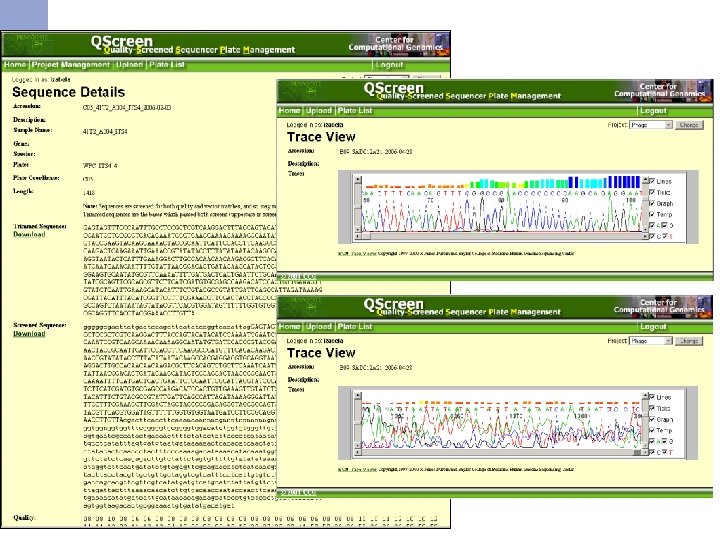
Qscreen n Sequencing data management and quality checking system Quality screening n Relational database for sequence data management and archive n Easy data access via web interface n Easy data sharing n Sequence and trace view n Project statistics n Password protected n

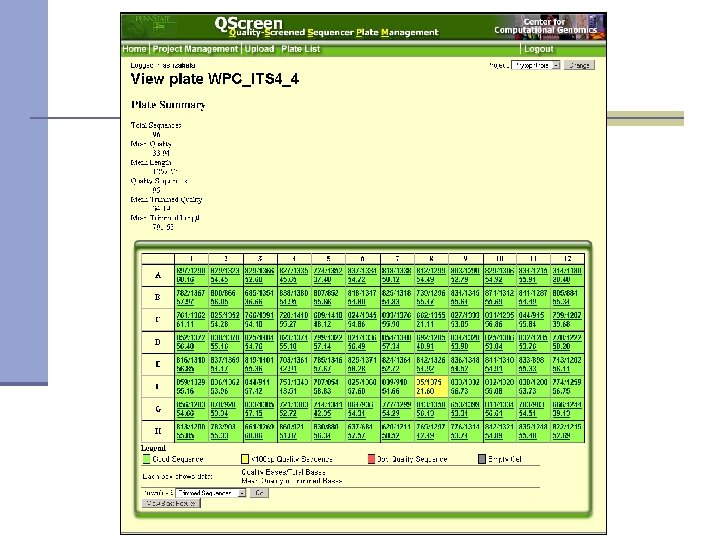
Qscreen: project and user management

Gene discovery strategy n Cluster and assemble EST sequences to lower redundancy and to increase the length of transcripts n Find coding regions and reading frame n Use deducted protein to search databases and assign function to the gene

Cluster and assemble EST resources n Assembly tools: TGICL http: //www. tigr. org/tdb/tgi/software/ n Cap 3 http: //genome. cs. mtu. edu/sas. html n Phrap http: //www. phrap. org/ n n EST clusters databases Uni. Gene http: //www. ncbi. nlm. nih. gov/ n TGI http: //www. tigr. org/ n n EST analysis pipeline n SMAPi http: //smapi. cbio. psu. edu

Assembling ESTs n Two stage process: n Clustering ESTs based on the similarity and clone ID n Assembling inside each cluster

Important parameters Length and similarity level of overlapping fragments Length of overhanging fragments n Criteria too stringent = many ESTs will not be assembled and genes will stay fragmented n Criteria too loose = ESTs from genes from the same family will be assembled into one gene

Contig quality ATGTCTCTNTCACTGA TCTGTCCC-CAGTCACGATCGAN ATGTCTCTGTCNCTNAGTCACGATCGAN ATGTCTCTNTCACTGA TCTGTCCC-CAGTCACGATCGAN ATGTCTCGGTCAC-CAGTCACGATCGAT TTGTCTGGGTCAC-CTCC GGTGGC-CAGTCACGATNGAN ATGTCTCGGTCAC-CAGTCACGAT ATGTCTCTGTCNCTNAGTCACGATCGAN ATGTCTCGGTCAC-CAGTCACGAT

One gene one cluster? Joined based on similarity 5’ESTs Joined based on clone ID Joined based on similarity 3’ESTs

One cluster one gene?

Cap 3 n Use of forward-reverse constraints to correct assembly errors and link contigs. n Use of base quality values in alignment of sequence reads. n Automatic clipping of 5' and 3' poor regions of reads. n Generation of assembly results in ‘ace’ file format for Consed.

Input files n CAP 3 takes as input a file of sequence reads in FASTA format. CAP 3 takes two optional files: a file of quality values in FASTA format and a file of forward-reverse constraints. The file of quality values must be named "xyz. qual", and the file of forward-reverse constraints must be named "xyz. con", where "xyz" is the name of the sequence file. CAP 3 uses the same format of a quality file as Phrap.

Web interface http: //bio. ifom-firc. it/ASSEMBLY/assemble. html

Output files

TGICL – TIGR Gene Indices clustering tool n Clustering – uses modified megablast program to cluster sequences together n Assembly – CAP 3 is used to assemble sequences inside each cluster

TGICL – TIGR Gene Indices clustering tool n Sequences need to be cleaned before using TGICL (Lucy, Uni. VEc, Seq. Clean) n m. RNA sequences may be used as ‘seeds’ for clustering. Caution: partial m. RNAs mislabeled as complete can prevent cluster extension beyond the seed. n Difficulty with highly expressed genes that have several thousand ESTs in a single cluster (assembly program may run out of memory)

Phrap n part of the Phred/Phrap/Consed n program for assembling shotgun DNA sequence data. n allows use of the entire read and not just the trimmed high n n n quality part uses a combination of user-supplied and internally computed data quality information to improve assembly accuracy constructs the contig sequence as a mosaic of the highest quality read segments rather than a consensus provides extensive assembly information to assist in troubleshooting assembly problems handles large datasets It is strongly recommended that phrap be used in conjunction with the base calls and base quality values produced by the basecaller, phred; and with the sequence editor/assembly viewer, consed.

Phrap output in Consed

Apple EST assembly 183, 732 ESTs n Phrap: n 24, 199 contigs; 9, 765 singletons n CAP 3 n 19, 791 contigs; 18, 927 singletons n TGICL n 22, 481 contigs; 28, 279 singletons

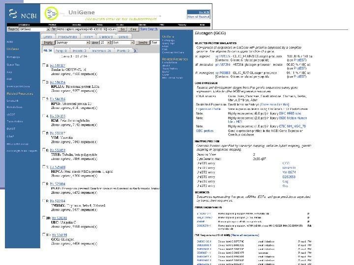
NCBI Uni. Gene

Clustering at NCBI n EST must have at least 100 bp after removing contaminants n The overlap between similar ESTs must be at least 70 bp n Similarity between overlapping area must be at least 96% over the 70% of overlapping region >100 bp >70% of overlap with at least 96% of similarity >100 bp >70 bp

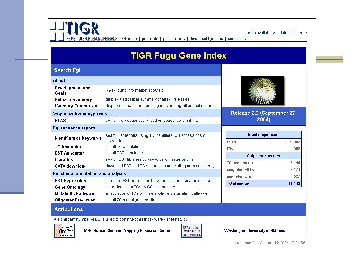
TIGR Gene Indices www. tigr. org

What are TIGR gene indices? n Clustered and assembled ESTs and m. RNA sequences n Each gene and each splice variant is represented by a single consensus sequence n Provides ORF annotation, genome mapping, expression profiles, domain annotation, unique oligomers <30 bp >40 bp of overlap with at least 95% of similarity <30 bp

TGI annotations

TGI sequence annotations

BLAST search

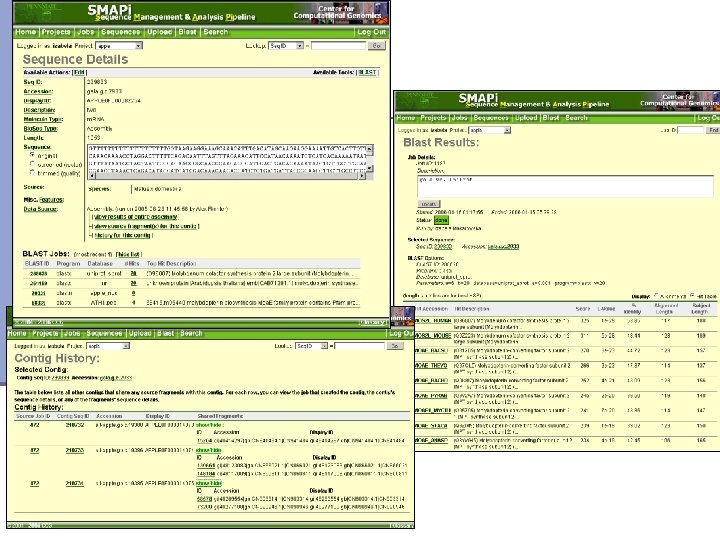
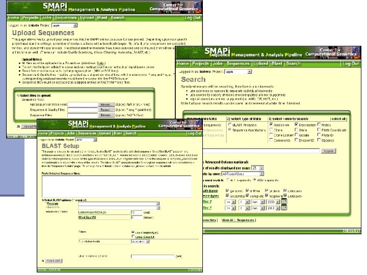
SMAPi – Sequence Management and Analysis Pipeline n The Parasitic Plant Genome Project Comparative genomics of related n Online access to data parasitic genera n Easy sequence management n Host-parasite lateral n Custom as well as automated transfer n annotation n Sharing among researchers n Integrated usage of various analysis tools (BLAST, Phred/Phrap. ) Supported by grant from Pennsylvania Greenhouse for Life Sciences

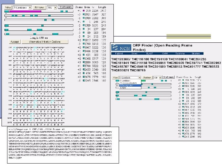
NCBI ORF finder

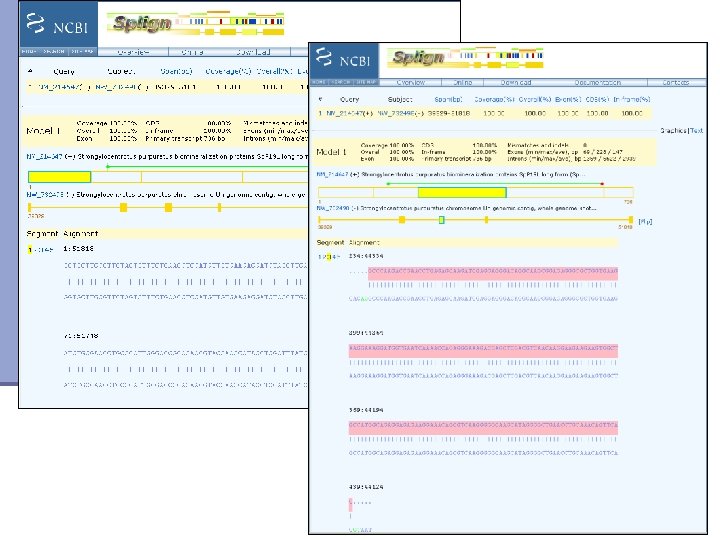
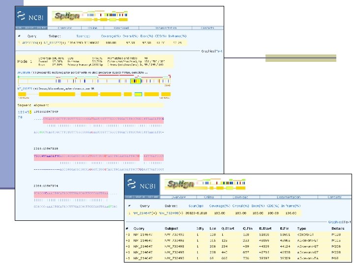
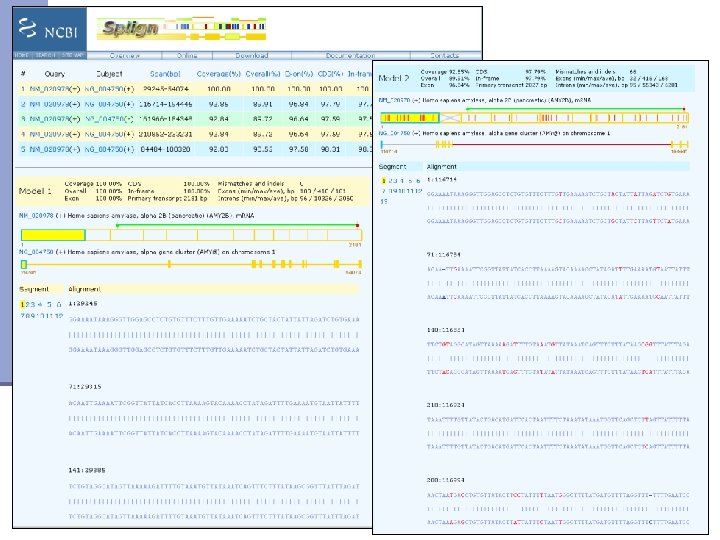
Mapping contigs to the genome n Splign http: //www. ncbi. nlm. nih. gov/sutils/splign/

Genome sequencing Access to entire genome n Regulatory elements n Only small percentage of the genome codes for genes n Hard to identify less typical genes n High rate of false positives n TGCATCGTAGCTAGCGCATGCTAGCTAGCTACGATGCATCGATGCTAGCTAGCATGCTAGCTATTGG CGCTAGCATGCATCGATGCATCGATTATAAGCGCGATGACGTCAG CGCGCGCATTATGCCGCGGCATGCTGCGCACAGTACTATAGCATTAGTAAAAA GGCCGCGTATATTTTACACGATAGTGCGGCGCGTAGCTAGTGCTAGTC TCCGGTTACACAGGTAGCTAGCTGCTAGCTGCTGCATGCATTAGT AGCTAGTGTAGCTAGCATGCTGCTAGCATGCATCGGGCGCGATGCT GCTAGCGCTGCTAGCTAGCTAGGCGCTAATTATTTTGGGGGGTTA AAAAATTTCGCTGCTTATACCCCCACATGATGATCGTTAGTAGCTACT AGCTCTCATCGCGCGGGGGGATGCTTAGCGTGGTGTGTGGTGTGGTC CTATAATTAGTGCATCGGCGCATCGATGGCTAGTCGATCGATTTTATATATCT AAAGACCCCATCTCTCTTTTCCCTTCTCTCGCTAGCGGTACGATTTACC

Genome sequencing strategies

Gene identification methods n Molecular techniques n Very laborious n Time consuming n Expensive n Low rate of false positives n Computational methods n Fast n Relatively low cost n High rate of false positives n Poor performance on less typical genes

Before we start analysis… n We have to: n Check sequences quality n Remove contamination n Assembly sequence reads into longer contigs n Close gaps (in perfect situation)

Gene finding strategies Genomic Sequence Model based Content-Based Bulk properties of sequence: Ÿ Open reading frame Ÿ Codon usage Ÿ Repeat periodicity Ÿ Compositional complexity Site-Based Absolute properties of sequence: Ÿ Consensus sequences Ÿ Donor and acceptor splice sites Ÿ Transcription factor binding sites Ÿ Polyadenylation signals Ÿ Start codon Ÿ Stop codon Comparative Inferences based on sequence homology: Ÿ Protein sequence with similarity to translated product of query Ÿ Similarity to EST sequences Ÿ Conserved regions between species (comparative genomics)

Gene finding methods classification Similarity based predictors: make use of similarity to already known genes and proteins coded by these genes as well as expression data including sequences from c. DNAs and data from hybridization experiments (tiling arrays for example) Dual- and multi-genome predictors: rely on the fact that functional regions of a genome sequence are more conserved during evolution Model based predictors: use a single genome sequence and exon/intron structure is predicted based on absolute and bulk properties of the sequence

Comparative genomics - Multi. Pipmaker http: //pipmaker. bx. psu. edu/pipmaker/

Model based methods n We take advantage of what we already learned about gene structures and features of coding sequences. Based on this knowledge we can build theoretical model, develop an algorithm to search for important features, train it on known data and use to search for coding sequences in anonymous genomic fragments

Pattern recognition and matching n The ability of a program to compare novel and known patterns and determine the degree of similarity forms the basis of sequence analysis including gene identification. In similarity based methods we search the genome directly for nucleotide or amino acid pattern observed in one or more already known genes; in comparative genomics we look for similar sequence pattern in two or more genomes, and in method based prediction we look for patterns in sequence composition and signals. n One of the major challenges associated with using pattern matching is in that, in most cases, we need to identify patterns that are ‘similar’ to a target pattern, but the concept of similarity isn’t well defined from programmatic and biological sense. Also, only already known pattern may be used for searches, therefore genes with unusual patterns may not be discovered using these methods.

Coding regions in Prokaryotes INTERGENIC REGION START CODING SEQUENCE STOP

Genetic code

Gene Model in Prokaryotes T A T G 1 START CODON 3 A T A G T 2 A G A STOP

Open Reading Frames +1 +2 +3 -1 -2 -3

Properties of the sequence n We can check if sequence in particular ORF has some other features which could tell us if this is a putative coding sequence or the ORF is false positive. We can look at the sequence content and compare it with known coding sequence and non-coding sequence and check to which of these two the ORF sequence is more similar to.

Markov chain n A Markov chain describes at successive times the states of a system. At these times the system may have changed from the state it was in the moment before to another or stayed in the same state. The changes of state are called transitions. The Markov property means the system is memoryless, i. e. it does not "remember" the states it was in before, just "knows" its present state, and hence bases its "decision" to which future state it will transit purely on the present, not considering the past.

Examples of Markov chain n A game of Monopoly, snakes and ladders or any other game whose moves are determined entirely by dice is a Markov chain. This is in contrast to card games such as poker or blackjack, where the cards represent a 'memory' of the past moves. To see the difference, consider the probability for a certain event in the game. In the above mentioned dice games, the only thing that matters is the current state of the board. The next state of the board depends on the current state, and the next roll of the dice. It doesn't depend on how things got to their current state. In a game such as poker or blackjack, a player can gain an advantage by remembering which hands have already been played (and hence which cards are no longer in the deck), so the next state (or hand) of the game is not independent of the past states.

Markov chain – weather model n The matrix P represents the weather model in which a sunny day is 90% likely to be followed by another sunny day, and a rainy day is 50% likely to be followed by another rainy day. 0. 1 0. 9 0. 5 P = 0. 9 0. 1 0. 5

Markov chain – sequence properties A T C G

How can we do this? CGATCGATCGGCCGATGCTGATGAGTCTCCTACGTCTCGTAGCTCGCGTCG TATATCGCGATCGCGTACGCGATCGCTATCTCGCATCGCGTACTGCAT CGATCGATCGATCGGCCGATGCTGATGAGTCTCCTACGTCTCGTAGCTCGCGTCG TATATCGCGATCGCATCGCGTACGCGATCGCATCTCGCATCGCGTACTGCAT CGATCGATCGGCCGATGCTGATGAGTCTCCTACGTCTCGTAGCTCGCGTCG TATATCGCGATCGCGTACGCGATCGCATCGCGTACTGCAT 20 G 7 GA 1 GG 5 GT 7 GC 7/20 1/20 5/20 7/20 For non-coding sequence we assume that probability of each is equal. The more ‘popular’ in coding sequence transition, the higher probability the sequence is coding

Markov Chains GCGCTAGCGCCGATCATCTACTCG GCGCTAGCGCCGATCATCTACTCG } } } first order second order fifth order

How far can we go? n Order of our model will have influence on specificity and sensitivity of our program. Too short sequences may not be specific enough and program may return a lot of false positives. Long chains may be to specific and our program will not be sensitive enough and will return a lot of false negatives.

Probability matrix first order Markov Model - matrix of 16 probabilities p(A/A), p(A/T), p(A/C), p(A/G) p(T/A), p(T/T), p(T/C), p(T/G) p(C/A), p(C/T), p(C/C), p(C/G) p(G/A), p(G/T), p(G/C), p(G/G) 4 4 1+1 4 K+1 2 = 4 =16 2+1 4 3+1 3 = 4 =64 4 =256

Probabilities in different reading frames GCGCTAGCGCCGATCATCTACTCG GCG CTA GCG CCG ATC TAC TCG G CGC TAG CGC CGA TCT ACT CG GC GCT AGC GCC GAT CTA CTC G Does G more often follow GC when it is in third position in codon or if it is in second or first position?

Number of probabilities 1+1 2 4 = 16 2 1+1 4 = 3 x 16 = 48

Estimating coding potential To estimate if the sequence is coding we have to calculate the probability that the sequence is coding and the probability the sequence is non-coding. Next we calculate the logarithm of the ratio of these two probability values i LP (S) = log P (S) P 0(S) If the calculated value is > 0 the likelihood that the sequence is coding is higher than the sequence is not coding. If the value is < 0 there is higher likelihood that sequence is not coding.

Markov Models - probabilities i LP(S) = log P (S) P 0(S) S=AGGACG 1 1 2 3 1 2 P(S) =f(A, 1)F(G, A)F(G, G)F(A, G)F(C, A)F(G, C) P(S) = 0. 27 x 0. 19 x 0. 27 x 0. 24 x 0. 21 x 0. 12 = 0. 00008377 P(S) = 0. 25 x 0. 25 =0. 0002441 LP(S) = log(0. 00008377/0. 0002441) = -0. 4644

Calculating LP i LP(S) = log P (S) P 0(S) 0. 27 0. 21 LP(S) = log 0. 27 + log 0. 19 + log 0. 24 + log 0. 12 0. 25 LP(S) = log 1. 08 + log 0. 76 + log 1. 08 + log 0. 96 + log 0. 84 + log 0. 48 LP(S) = 0. 0334 + (-0. 1191) +0. 0334 + (-0. 0177) + (-0. 0757) + (-0. 3187) LP(S) = -0. 4644

GLIMMER n. Gene finding program for Prokaryotes n. Saltzberg et. al, 1998 n. For prediction uses: n. Start n. Stop n. Sequence composition n. Interpolated Markov Models

The GLIMMER system n Part 1 – Program is trained for given data set (species) n Part 2 – Program identifies putative genes in the genomic sequence n Identify all ORFs longer than a threshold n Score each ORF in each reading frame and select these which gets highest scores in correct reading frame n Score overlapping genes in each frame separately to see which frame score the highest

Running the program n First run build-imm on a set of sequences to make the Markov models (long ORFs from the same or closely related species) nbuild-imm train. seq n Then run GLIMMER to find genes in your sequence nglimmer your. seq train. seq <options>

GLIMMER options n -g set minimum gene length n -o set minimum overlap n -p set minimum overlap percentage n +r/-r independent probability score ON/OFF n -t set threshold score for calling as gene

GLIMMER output Minimum gene length = 180 Minimum overlap length = 30 Minimum overlap percent = 10. 0% Threshold score = 90 Use independent scores = True Use first start codon = True ID# 1 2 3 4 *** 5 *** 6 7 8 Orf Fr Start F 2 302 R 1 660 F 2 620 R 3 1114 F 3 1119 R 3 2026 F 3 1815 Overlaps #3 Reject #4 R 2 2600 Overlaps #4 F 1 2710 R 3 4153 F 1 3403 R 2 4700 R 2 68906 R 1 101574 R 3 193228 Gene Start 305 633 650 1105 1140 1999 1830 by 170 2597 by 120 2719 4153 3403 4679 68897 101544 193204 End 616 220 901 638 1466 1118 2054 1935 3399 3962 4230 4455 68670 101296 193022 Lengths Gene -- Frame Orf Gene Score F 1 F 2 F 3 315 312 0 _ 441 414 99 _ _ _ 282 252 0 _ 477 468 99 _ _ _ 348 327 0 _ _ 0 909 882 99 _ _ _ 240 225 99 _ _ 99 Overlap Region Scores: _ _ 0 666 Overlap 690 192 828 246 237 279 207 663 99 _ Region Scores: _ 681 99 99 192 0 99 828 99 99 225 0 _ 228 13 _ 249 96 _ 183 56 _ _ _ _ _ Scores R 1 R 2 R 3 99 _ _ _ _ 99 _ _ _ 99 _ 0 _ 99 _ _ _ _ 0 _ _ _ 13 _ _ 96 _ _ _ 56 Indep Score 0 0 0 0 99 86 3 43

List of putative genes Putative Genes: 1 633 220 2 1105 638 3 1999 1118 5 2597 1935 6 2719 3399 7 3403 4230. . . 39 38472 38741 [Shorter 40 80 74] 40 38662 39450 [Bad Overlap 39 80 25]. . . 482 464206 464424 [Shadowed by 483]. . . 636 616213 615965 [Delay by 33 637 50 0]

Output description 39 40 38472 38662 38741 [Shorter 40 80 74] 39450 [Bad Overlap 39 80 25] [Bad Overlap a b c] means that gene number a overlapped this one and was shorter but scored higher on the overlap region. b is the length of the overlap region and c is the score of *this* gene on the overlap region. There should be a [Shorter. . . ] notation with gene a giving its score. [Shorter a b c] means that gene number a overlapped this one and was longer but scored lower on the overlap region. b is the length of the overlap region and c is the score of *this* gene on the overlap region. There should be a [Bad overlap. . . ] notation with gene a giving its score.

Output description - 2 482 464206 464424 [Shadowed by 483]. . . 636 616213 615965 [Delay by 33 637 50 0] [Shadowed by a] means that this gene was completed contained as part of gene a 's region, but in another frame. [Delay by a b c d] means that this gene was tentatively rejected because of an overlap with gene b , but if the start codon is postponed by a positions, then this would be a valid gene. The start position reported for this gene includes the delay. c is the length of the overlap region that caused the rejection and d is the score in this gene's frame on that overlap region.

Prokaryotic vs. Eukaryotic Genes n Prokaryotes n Eukaryotes n small genomes n large genomes n high gene density n low gene density n no introns (or splicing) n introns (splicing) n no RNA processing n similar promoters n heterogeneous promoters n terminators important n terminators not important n overlapping genes n polyadenylation

Coding regions in Prokaryotes INTERGENIC REGION START CODING SEQUENCE STOP

From DNA to protein

Gene structure

Pseudogenes and repetitive elements

Complicated gene structures

Overlapping genes

Eukaryotic gene structure

3’ UTR 5’ UTR Ex 1 In 1 Ex 2 In 2 Ex 3 In 3 GT AG Ex 4 In 4 Ex 5 E 0 E 2 I 0 Markov Models E 1 I 2 Eterm Einit 5’ UTR Single exon gene 3’ UTR Poly A promoter Signal Intergenic region Ex 5

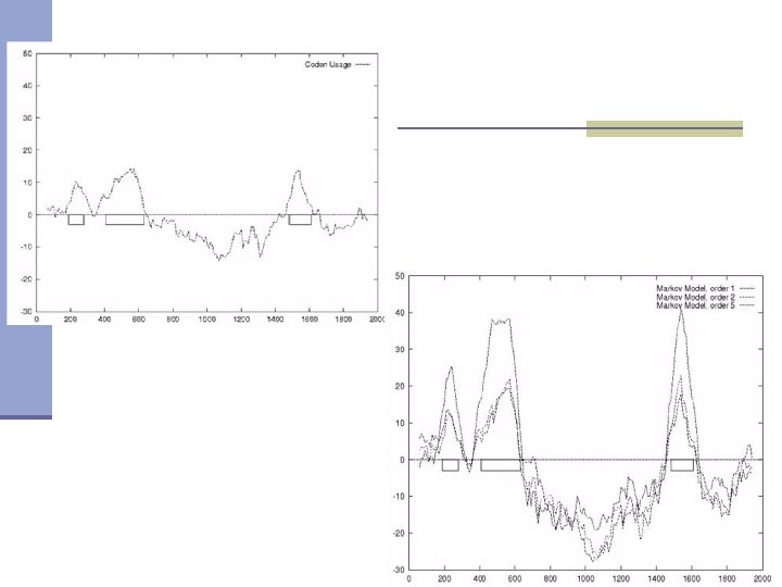
Searching for coding sequences using Markov chain In this case we do not want check if given sequence fragment is coding or not but we rather want to identify coding fragments in a long sequence. In most cases this is done by calculating statistics in overlapping windows. AGTACGATATTAGCGGCAATCGTATGACTACGTCTTGCTACGTCTTCTCTCGTCTGCTCTAG Windows coding potentials are used to create profiles. This example shows a profile for a sequence analyzed using 120 bp windows with 10 bp distance between them.

Codon usage

Probability that sequence is coding

Probability that sequence is non-coding

Log-likelihood ratio

Rule based method Neural network

GRAIL n n Gene recognition and Analysis Internet Link Uberbacher and Mural, 1991 First gene prediction program GRAIL 1 n n Neural network recognizing coding potential within fixed-size window (100 bp) Evaluates coding potential without looking for additional features (e. g. splice junctions, start and stop codons) n GRAIL 2 n Variable size of windows n Incorporated genomic context information (splice sites, start and stop, polyadenylation signals) n GRAILEXP n http: //compbio. ornl. gov/grailexp/

GRAILEXP

MZEF n M. Zhang 1997 n Predicts exons only, does not build gene structure n Uses ‘quadratic discriminant analysis” n Variable measures: n Exon length n Intron-exon transition n Branch site scores n http: //rulai. cshl. org/tools/genefinder/

MZEF

FGENES n Solovyev et al. , 1994 n Predicts internal exons n Linear discriminant analysis n Donor and acceptor splice sites n Putative coding regions n Intronic regions both 5’ and 3’ to the putative exon n Passes results to a dynamic programming algorithm to come up with coherent gene model n http: //www. softberry. com/berry. phtml

FGENESH

GENSCAN n Burge and Karlin n Search for general and specific compositional properties of distinct functional units in eukaryotic genes n General fifth-order markov model of coding regions n Analyze both DNA strands n Sequences may contain multiple and/or partial genes n http: //genes. mit. edu/GENSCAN

GENSCAN options

GENSCAN output

Graphical output

Are predictions the same? GRAILEXP MZEF FGENESH Gen. Scan

Evaluation statistic TP TP - true positive FP - false positive FN - false negative TN - true negative FP FN TN TP

Experimental validation of predicted genes Ÿ not annotated human BAC clones 20 Ÿ finished 3 Ÿ unfinished 17 Ÿ Genes that had at least two exons, each predicted by at least two programs Ÿ the overlap of the predicted exons did not have to be perfect Ÿ similarity to ESTs or known genes was used as supporting evidence but was not required Ÿ genes (number of exons 2 -11) 40 Ÿ Six single exons predicted by three or four programs Ÿ Three two-exon genes predicted by one program only but strongly supported by similarities to EST sequences Ÿ genes were eliminated from further studies as they contained 12 repetitive elements and were most likely false positives Ÿ Total: 37 putative transcripts

Prediction programs performance 37 genes were tested, 16 of them (43%) were confirmed. At the exon level there were 159 exons and 58 (36%) were found to be real predicted exons specificity sensitivity MZEF 34 0. 51 0. 56 GRAIL 11 0. 48 0. 19 GENSCAN 52 0. 46 0. 91 FGENES 45 0. 37 0. 75

Gene structure and alternative splicing

Repetitive elements 12 genes containing large fragments of repetitive elements were eliminated from experimental validation. However some proteins are partially coded by Alu or MER (Makalowski 1994, 2000) Gene gm 121 contains MER at 5' end of c. DNA and this is experimentally confirmed gene. Gene gm 124 was eliminated from our experimental validation based on the presence of repetitive element. Further analysis showed that this gene is a part of transcript FLJ 23129, Gen. Bank accession AK 026782

Repetitive elements Ÿ 50% of mammalian genome are repeats: Ÿ DNA transposons Ÿ retrotransposons Ÿ LINEs Ÿ SINEs Ÿ tandem repeats Ÿ masking before similarity search - helps avoid getting similarities caused by the presence of repetitive elements, not because of sequences homology Ÿ predicted gene with repetitive elements are less likely to be real, although sometimes repeats are true parts of coding sequence

Repeat. Masker Ÿ Searches for Alu, MIR, LINE, LTR and other repeats by comparison to sequences in Rep. Base library Ÿ Rep. Base is a database of repetitive DNA sequence elements found in a variety of eukaryotic organisms including primates, rodents, cow, dog, chicken, fugu, drosophila, arabidopsis, rice Ÿ Accepts local databases with repetitive elements Ÿ Repetitive elements are masked by replacing nucleotides with string of letters N Ÿ Masking can be limited to certain types of repeats only

Repeat. Masker http: //www. repeatmasker. org/

Repeat. Masker outputs

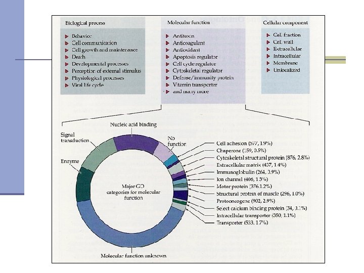
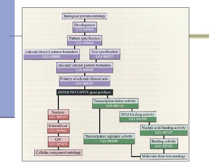
Functional annotation- Gene Ontology n Gene Ontology: A controlled vocabulary to describe gene products - proteins and RNA - in any organism. n Gene is described in three categories: n Cellular component: where a gene product acts Molecular function: activities or “jobs” of a gene product n Biological process: a commonly recognized series of events n

Annotation source ISS IDA IPI TAS NAS IMP IGI IEP IC ND Inferred from Sequence/Structural Similarity Inferred from Direct Assay Inferred from Physical Interaction Traceable Author Statement Non-traceable Author Statement Inferred from Mutant Phenotype Inferred from Genetic Interaction Inferred from Expression Pattern Inferred by Curator No Data available IEA Inferred from electronic annotation

Gene annotation

Annotating genes n Model organism: look at curated databases

Annotating novel genes n Similarity search against curated and well annotated database: functional annotations deducted from close and significant match n Functional domains identification: mapping domains and terms to Gene Ontology

Annotating novel genes n Similarity search against curated and well annotated database: functional annotations deducted from close and significant match n Identification of functional domains: mapping domain to GO term

Regulatory sequences n Difficult to identify using computer programs n Most regulatory elements are still not identified n They are usually very short: 6 -10 base pairs n They may differ in one or more places

Finding regulatory elements n Phylogenetic footprinting – comparative genomics used to identify conserved non-coding sequences (Multi. Pip. Maker) n Phylogenetic shadowing – conceptually similar to phylogenetic footprinting, with the difference that closely related species are compared (e. Shadow) n Gibbs sampling – random iterations of the promoter regions alignments to identify blocks of conserved residues (Gibbs Motif Sampler) n Hidden Markov Models – searching for known regulatory elements using probability matrices (Cister)

Phylogenetic shadowing

Gibbs sampling ACGGTACGTTGG GGTACGTAGGAC TGGCTACCTTGG CGGTACGTAGGT ******* **

Building model from existing alignment ACA TCA AGA ACC --ACT C---G-- ATG ATC AGC ATC insertion Transition probabilities Output Probabilities A HMM model for a DNA motif alignments, The transitions are shown with arrows whose thickness indicate their probability. In each state, the histogram shows the probabilities of the four bases.

Cister Ÿ Detects cis-elements clusters by using Hidden Markov Model Ÿ For each element uses separate matrix with frequencies of each nucleotide in each position; user can input matrix for elements not included in the basic option Ÿ User can specify: ƒ distance between neighboring cis-elements within a cluster ƒ number of cis-elements in the cluster ƒ distance between clusters ƒ half-width of the sliding window

Frequency matrix NA AML-1 a XX DE runt-factor AML-1 XX BF T 02256; AML 1 a; Species: human, sapiens. XX P 0 A C G T 01 5 1 2 49 02 2 2 52 1 03 4 14 1 38 04 0 0 57 0 05 1 0 55 1 06 1 4 0 52 Homo T G G T TGTGGT TGCGGT TGTGGT AGTGGT TGTGGC Sequences of experimentaly identified elements are aligned and frequencies in each position are calculated

Cister http: //zlab. bu. edu/~mfrith/cister. shtml