Computational Gene Finding using HMMs Nagiza F Samatova

Computational Gene Finding using HMMs Nagiza F. Samatova Computational Biology Institute Oak Ridge National Laboratory samatovan@ornl. gov

Outline Ø Gene Finding Problem Ø Simple Markov Models Ø Hidden Markov Models Ø Viterbi Algorithm Ø Parameter Estimation Ø GENSCAN Ø Performance Evaluation

Gene Finding Problem Ø General task: § to identify coding and non-coding regions from DNA § Functional elements of most interest: promoters, splice sites, exons, introns, etc. Ø Classification task: § Gene finding is a classification task: X X Ø Observations: nucleotides Classes: labels of functional elements Computational techniques: § § Neural networks Discriminant analysis Decision trees Hidden Markov Models (HMMs) Focus of today’s lecture

General Complications Ø Not all organisms use the same genetic code: § But computational methods are usually “tuned” for some set of organisms Ø Overlapping genes (esp. , in viruses): § Genes encoded in different reading fames on the same or on the complementary DNA Ø Prokaryotic vs. Eukaryotic genes

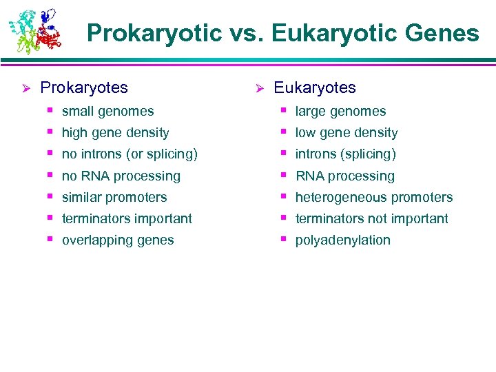Prokaryotic vs. Eukaryotic Genes Ø Prokaryotes § § § § small genomes high gene density no introns (or splicing) no RNA processing similar promoters terminators important overlapping genes Ø Eukaryotes § § § § large genomes low gene density introns (splicing) RNA processing heterogeneous promoters terminators not important polyadenylation

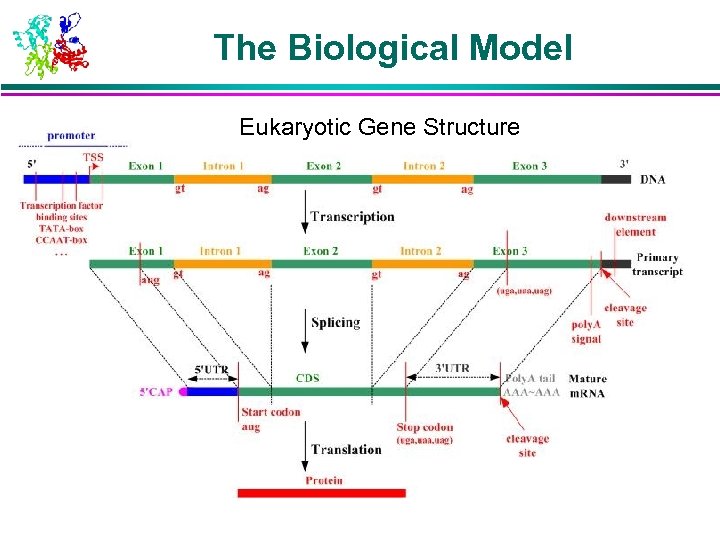The Biological Model Eukaryotic Gene Structure

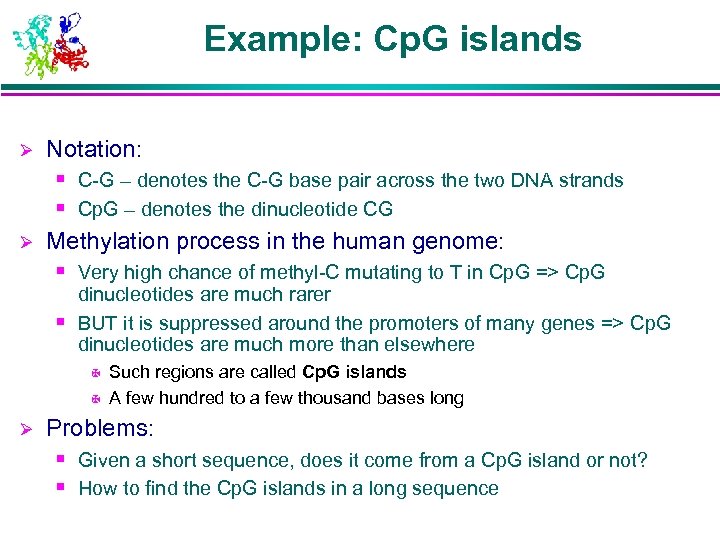Example: Cp. G islands Ø Notation: § C-G – denotes the C-G base pair across the two DNA strands § Cp. G – denotes the dinucleotide CG Ø Methylation process in the human genome: § Very high chance of methyl-C mutating to T in Cp. G => Cp. G dinucleotides are much rarer § BUT it is suppressed around the promoters of many genes => Cp. G dinucleotides are much more than elsewhere X X Ø Such regions are called Cp. G islands A few hundred to a few thousand bases long Problems: § Given a short sequence, does it come from a Cp. G island or not? § How to find the Cp. G islands in a long sequence

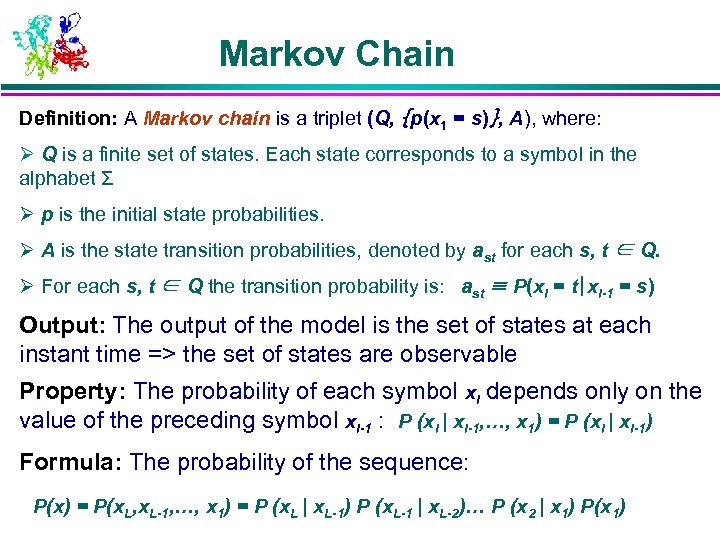Markov Chain Definition: A Markov chain is a triplet (Q, {p(x 1 = s)}, A), where: Ø Q is a finite set of states. Each state corresponds to a symbol in the alphabet Σ Ø p is the initial state probabilities. Ø A is the state transition probabilities, denoted by ast for each s, t ∈ Q. Ø For each s, t ∈ Q the transition probability is: ast ≡ P(xi = t|xi-1 = s) Output: The output of the model is the set of states at each instant time => the set of states are observable Property: The probability of each symbol xi depends only on the value of the preceding symbol xi-1 : P (xi | xi-1, …, x 1) = P (xi | xi-1) Formula: The probability of the sequence: P(x) = P(x. L, x. L-1, …, x 1) = P (x. L | x. L-1) P (x. L-1 | x. L-2)… P (x 2 | x 1) P(x 1)

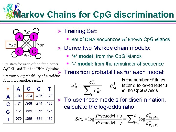Markov Chains for Cp. G discrimination A a. AT Ø T a. AC Training Set: § set of DNA sequences w/ known Cp. G islands a. GT Ø C a G GC • A state for each of the four letters A, C, G, and T in the DNA alphabet Ø • Arrow <-> probability of a residue following another residue + A C G T A . 180 . 274 . 426 . 120 C . 171 . 368 . 274 . 188 G . 161 . 339 . 375 . 125 T . 079 . 355 . 384 . 182 Ø Derive two Markov chain models: § ‘+’ model: from the Cp. G islands § ‘-’ model: from the remainder of sequence Transition probabilities for each model: is the number of times letter t followed letter s in the Cp. G islands To use these models for discrimination, calculate the log-odds ratio:

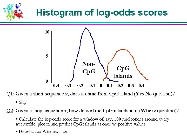Histogram of log-odds scores 10 5 Non. Cp. G 0 -0. 4 -0. 3 -0. 2 -0. 1 Cp. G islands 0 0. 1 0. 2 0. 3 0. 4 Q 1: Given a short sequence x, does it come from Cp. G island (Yes-No question)? • S(x) Q 2: Given a long sequence x, how do we find Cp. G islands in it (Where question)? • Calculate the log-odds score for a window of, say, 100 nucleotides around every nucleotide, plot it, and predict Cp. G islands as ones w/ positive values • Drawbacks: Window size

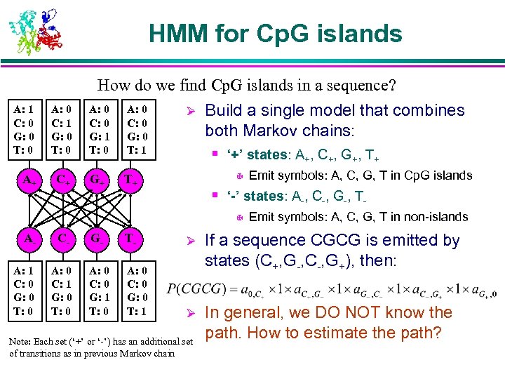HMM for Cp. G islands How do we find Cp. G islands in a sequence? A: 1 C: 0 G: 0 T: 0 A: 0 C: 1 G: 0 T: 0 A: 0 C: 0 G: 1 T: 0 A: 0 C: 0 G: 0 T: 1 A+ C+ G+ T+ Ø Build a single model that combines both Markov chains: § ‘+’ states: A+, C+, G+, T+ X Emit symbols: A, C, G, T in Cp. G islands § ‘-’ states: A-, C-, G-, TX Emit symbols: A, C, G, T in non-islands A- C- G- T- Ø A: 1 C: 0 G: 0 T: 0 A: 0 C: 1 G: 0 T: 0 A: 0 C: 0 G: 1 T: 0 A: 0 C: 0 G: 0 T: 1 If a sequence CGCG is emitted by states (C+, G-, C-, G+), then: Ø In general, we DO NOT know the path. How to estimate the path? Note: Each set (‘+’ or ‘-’) has an additional set of transitions as in previous Markov chain

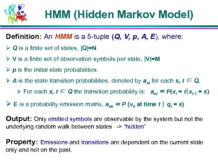HMM (Hidden Markov Model) Definition: An HMM is a 5 -tuple (Q, V, p, A, E), where: Ø Q is a finite set of states, |Q|=N Ø V is a finite set of observation symbols per state, |V|=M Ø p is the initial state probabilities. Ø A is the state transition probabilities, denoted by ast for each s, t ∈ Q. Ø For each s, t ∈ Q the transition probability is: ast ≡ P(xi = t|xi-1 = s) Ø E is a probability emission matrix, esk ≡ P (vk at time t | qt = s) Output: Only emitted symbols are observable by the system but not the underlying random walk between states -> “hidden” Property: Emissions and transitions are dependent on the current state only and not on the past.

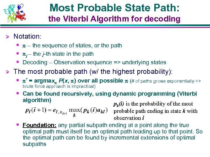Most Probable State Path: the Viterbi Algorithm for decoding Ø Notation: § – the sequence of states, or the path § j – the j-th state in the path § Decoding – Observation sequence => underlying states Ø The most probable path (w/ the highest probability): § * = argmax P(x, ) over all possible (# of paths grows exponentially => brute force approach is impractical) § Can be found recursively, using dynamic programming (Viterbi algorithm) pk(i) is the probability of the most probable path ending in state k with observation i § Foundation: any partial subpath ending at a point along the true optimal path must itself be an optimal path leading up to that point. So the optimal path can be found by incremental extensions of optimal subpaths

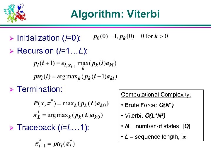Algorithm: Viterbi Ø Initialization (i=0): Ø Recursion (i=1…L): Ø Termination: Computational Complexity: • Brute Force: O(NL) • Viterbi: O(L*N 2) Ø Traceback (i=L… 1): • N – number of states, |Q| • L – sequence length, |x|

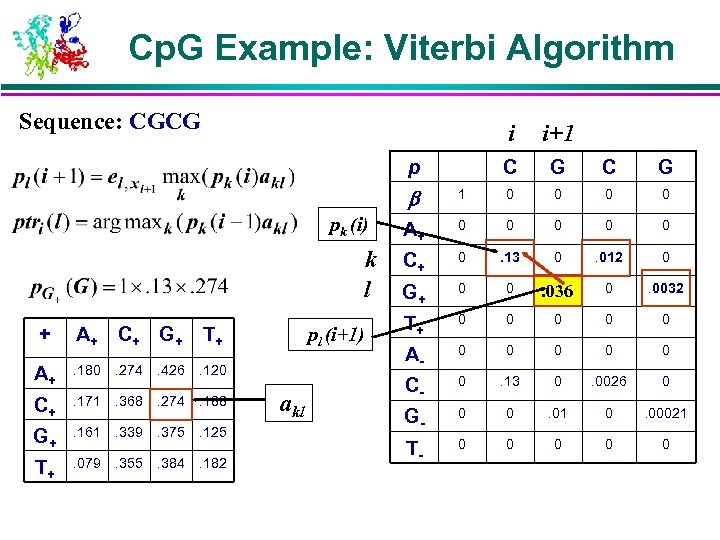Cp. G Example: Viterbi Algorithm Sequence: CGCG i C p i+1 G C G pk (i) k l + A+ C+ G + T+ A+ . 180 . 274 . 426 . 120 C+ . 171 . 368 . 274 . 188 G+ . 161 . 339 . 375 . 125 T+ . 079 . 355 . 384 . 182 pl (i+1) akl 1 0 0 A+ 0 0 0 C+ 0 . 13 0 . 012 0 G+ 0 0 . 034. 036 0 . 0032 T+ 0 0 0 A- 0 0 0 C- 0 . 13 0 . 0026 0 G- 0 0 . 01 0 . 00021 T- 0 0 0

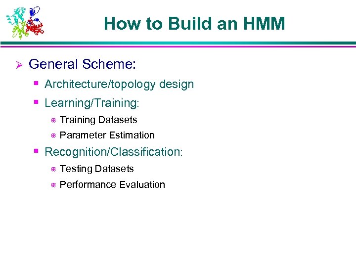How to Build an HMM Ø General Scheme: § Architecture/topology design § Learning/Training: X Training Datasets X Parameter Estimation § Recognition/Classification: X Testing Datasets X Performance Evaluation

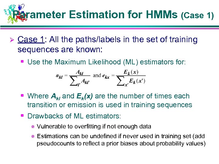Parameter Estimation for HMMs (Case 1) Ø Case 1: All the paths/labels in the set of training sequences are known: § Use the Maximum Likelihood (ML) estimators for: § Where Akl and Ek(x) are the number of times each transition or emission is used in training sequences § Drawbacks of ML estimators: X Vulnerable to overfitting if not enough data X Estimations can be undefined if never used in training set (add pseudocounts to reflect a prior biases about probability values)

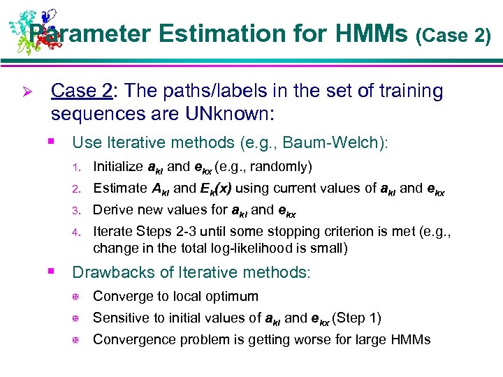Parameter Estimation for HMMs (Case 2) Ø Case 2: The paths/labels in the set of training sequences are UNknown: § Use Iterative methods (e. g. , Baum-Welch): 1. Initialize akl and ekx (e. g. , randomly) 2. Estimate Akl and Ek(x) using current values of akl and ekx 3. Derive new values for akl and ekx 4. Iterate Steps 2 -3 until some stopping criterion is met (e. g. , change in the total log-likelihood is small) § Drawbacks of Iterative methods: X Converge to local optimum X Sensitive to initial values of akl and ekx (Step 1) X Convergence problem is getting worse for large HMMs

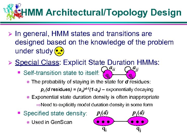HMM Architectural/Topology Design Ø In general, HMM states and transitions are designed based on the knowledge of the problem under study Ø Special Class: Explicit State Duration HMMs: aii ajj § Self-transition state to itself: qi qj X The probability of staying in the state for d residues: pi (d residues) = (aii)d-1(1 -aii) – exponentially decaying X Exponential state duration density is often inappropriate ÞNeed to explicitly model duration density in some form § Specified state density: X Used in Gen. Scan pi(d) … qi pj(d) … qj

HMM-based Gene Finding Ø GENSCAN (Burge 1997) Ø FGENESH (Solovyev 1997) Ø HMMgene (Krogh 1997) Ø GENIE (Kulp 1996) Ø GENMARK (Borodovsky & Mc. Ininch 1993) Ø VEIL (Henderson, Salzberg, & Fasman 1997)

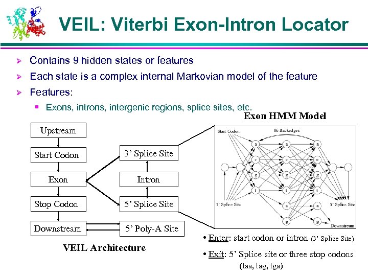VEIL: Viterbi Exon-Intron Locator Ø Contains 9 hidden states or features Ø Each state is a complex internal Markovian model of the feature Ø Features: § Exons, introns, intergenic regions, splice sites, etc. Exon HMM Model Upstream Start Codon 3’ Splice Site Exon Intron Stop Codon 5’ Splice Site Downstream 5’ Poly-A Site VEIL Architecture • Enter: start codon or intron (3’ Splice Site) • Exit: 5’ Splice site or three stop codons (taa, tag, tga)

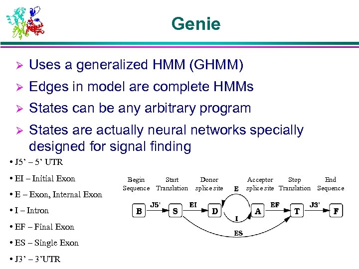Genie Ø Uses a generalized HMM (GHMM) Ø Edges in model are complete HMMs Ø States can be any arbitrary program Ø States are actually neural networks specially designed for signal finding • J 5’ – 5’ UTR • EI – Initial Exon • E – Exon, Internal Exon • I – Intron • EF – Final Exon • ES – Single Exon • J 3’ – 3’UTR Begin Start Sequence Translation Donor splice site Acceptor Stop End splice site Translation Sequence

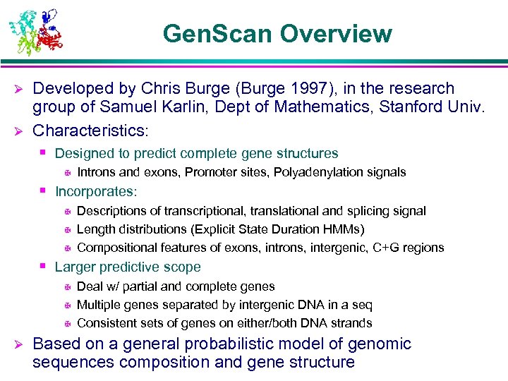Gen. Scan Overview Ø Ø Developed by Chris Burge (Burge 1997), in the research group of Samuel Karlin, Dept of Mathematics, Stanford Univ. Characteristics: § Designed to predict complete gene structures X Introns and exons, Promoter sites, Polyadenylation signals § Incorporates: X X X Descriptions of transcriptional, translational and splicing signal Length distributions (Explicit State Duration HMMs) Compositional features of exons, introns, intergenic, C+G regions § Larger predictive scope X X X Ø Deal w/ partial and complete genes Multiple genes separated by intergenic DNA in a seq Consistent sets of genes on either/both DNA strands Based on a general probabilistic model of genomic sequences composition and gene structure

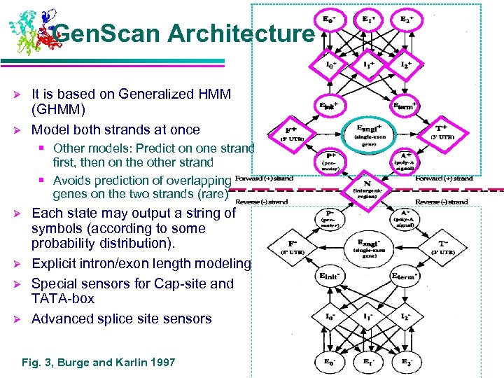Gen. Scan Architecture Ø Ø It is based on Generalized HMM (GHMM) Model both strands at once § Other models: Predict on one strand first, then on the other strand § Avoids prediction of overlapping genes on the two strands (rare) Ø Ø Each state may output a string of symbols (according to some probability distribution). Explicit intron/exon length modeling Special sensors for Cap-site and TATA-box Advanced splice site sensors Fig. 3, Burge and Karlin 1997

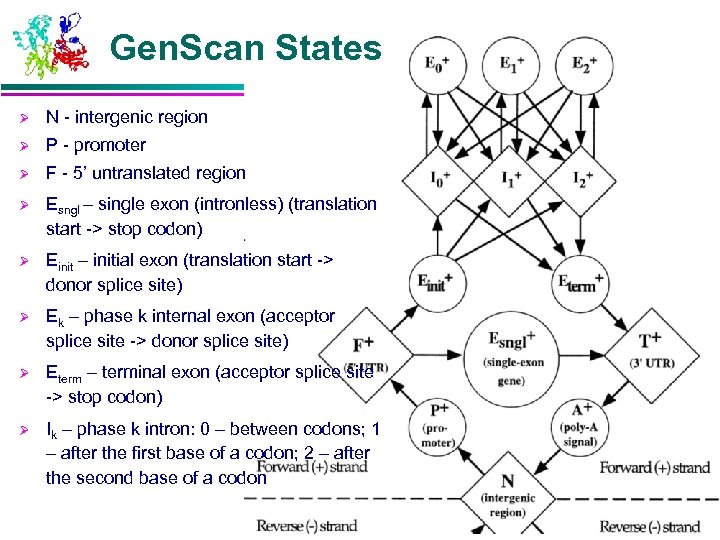Gen. Scan States Ø N - intergenic region Ø P - promoter Ø F - 5’ untranslated region Ø Esngl – single exon (intronless) (translation start -> stop codon) Ø Einit – initial exon (translation start -> donor splice site) Ø Ek – phase k internal exon (acceptor splice site -> donor splice site) Ø Eterm – terminal exon (acceptor splice site -> stop codon) Ø Ik – phase k intron: 0 – between codons; 1 – after the first base of a codon; 2 – after the second base of a codon

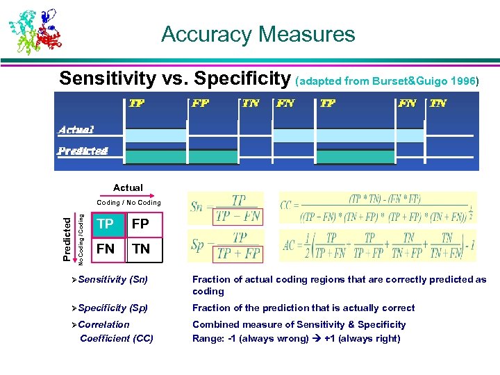Accuracy Measures Sensitivity vs. Specificity (adapted from Burset&Guigo 1996) TP FP TN FN TP FN TN Actual Predicted Actual No Coding / Coding Predicted Coding / No Coding TP FP FN TN ØSensitivity (Sn) Fraction of actual coding regions that are correctly predicted as coding ØSpecificity (Sp) Fraction of the prediction that is actually correct ØCorrelation Coefficient (CC) Combined measure of Sensitivity & Specificity Range: -1 (always wrong) +1 (always right)

Test Datasets Ø Sample Tests reported by Literature § Test on the set of 570 vertebrate gene seqs (Burset&Guigo 1996) as a standard for comparison of gene finding methods. § Test on the set of 195 seqs of human, mouse or rat origin (named HMR 195) (Rogic 2001).

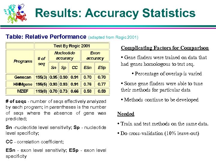Results: Accuracy Statistics Table: Relative Performance (adapted from Rogic 2001) Complicating Factors for Comparison • Gene finders were trained on data that had genes homologous to test seq. • Percentage of overlap is varied • Some gene finders were able to tune their methods for particular data # of seqs - number of seqs effectively analyzed by each program; in parentheses is the number of seqs where the absence of gene was predicted; Sn -nucleotide level sensitivity; Sp - nucleotide level specificity; CC - correlation coefficient; ESn - exon level sensitivity; ESp - exon level specificity • Methods continue to be developed Needed • Train and test methods on the same data. • Do cross-validation (10% leave-out)

Why not Perfect? Ø Gene Number usually approximately correct, but may not Ø Organism primarily for human/vertebrate seqs; maybe lower accuracy for nonvertebrates. ‘Glimmer’ & ‘Gene. Mark’ for prokaryotic or yeast seqs Ø Exon and Feature Type Internal exons: predicted more accurately than Initial or Terminal exons; Exons: predicted more accurately than Poly-A or Promoter signals Ø Biases in Test Set (Resulting statistics may not be representative) The Burset/Guigó (1996) dataset: Ø Biased toward short genes with relatively simple exon/intron structure The Rogic (2001) dataset: Ø Ø DNA seqs: Gen. Bank r-111. 0 (04/1999 <- 08/1997); source organism specified; consider genomic seqs containing exactly one gene; seqs>200 kb were discarded; m. RNA seqs and seqs containing pseudo genes or alternatively spliced genes were excluded.

What We Learned… Ø Genes are complex structures which are difficult to predict with the required level of accuracy/confidence Ø Different HMM-based approaches have been successfully used to address the gene finding problem: § Building an architecture of an HMM is the hardest part, it should be biologically sound & easy to interpret § Parameter estimation can be trapped in local optimum Ø Viterbi algorithm can be used to find the most probable path/labels Ø These approaches are still not perfect

Thank You!