Computational Game Theory What is Game Theory History

Computational Game Theory: What is Game Theory? History Mechanism Design Auctions Risk and Utility Pure and Mixed Zero Sum Games Minimax and LP formulation Yao’s Theorem Strongly based on Slides by Vincent Conitzer of Duke Modified/Corrupted/Added to by Michal Feldman and Amos Fiat

What is game theory? • Game theory studies settings where multiple parties (agents) each have – different preferences (utility functions), – different actions that they can take • Each agent’s utility (potentially) depends on all agents’ actions – What is optimal for one agent depends on what other agents do • Very circular! • Game theory studies how agents can rationally form beliefs over what other agents will do, and (hence) how agents should act – Useful for acting as well as predicting behavior of others

Where is game theory used? • Economics (& business) – Auctions, exchanges, price/quantity setting by firms, bargaining, funding public goods, … • Political science – Voting, candidate positioning, … • Biology – Stable proportions of species, sexes, behaviors, … • And of course… Computer science! – Game playing programs, electronic marketplaces, networked systems, … – Computing the solutions that game theory prescribes

A brief history of game theory • Some isolated early instances of what we would now call game-theoretic reasoning – e. g. Haldegrave 1713, Cournot 1838 • von Neumann wrote a key paper in 1928 • 1944: Theory of Games and Economic Behavior by von Neumann and Morgenstern • 1950: Nash invents concept of Nash equilibrium • Game theory booms after this… • 1994: Harsanyi, Nash, and Selten win Riksbank Prize (aka Nobel Prize) in economics for game theory work • 2005: Aumann and Schelling win Riksbank Prize (aka Nobel Prize) in economics for game theory work • 2007: Hurwicz, Maskin, and Myerson win Riksbank Prize (aka Nobel Prize) in economics for game theory work

What is mechanism design? • In mechanism design, we get to design the game (or mechanism) – e. g. the rules of the auction, marketplace, election, … • Goal is to obtain good outcomes when agents behave strategically (game-theoretically) • Mechanism design often considered part of game theory • Sometimes called “inverse game theory” – In game theory the game is given and we have to figure out how to act – In mechanism design we know how we would like the agents to act and have to figure out the game

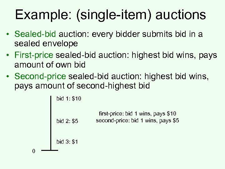Example: (single-item) auctions • Sealed-bid auction: every bidder submits bid in a sealed envelope • First-price sealed-bid auction: highest bid wins, pays amount of own bid • Second-price sealed-bid auction: highest bid wins, pays amount of second-highest bid 1: $10 bid 2: $5 bid 3: $1 0 first-price: bid 1 wins, pays $10 second-price: bid 1 wins, pays $5

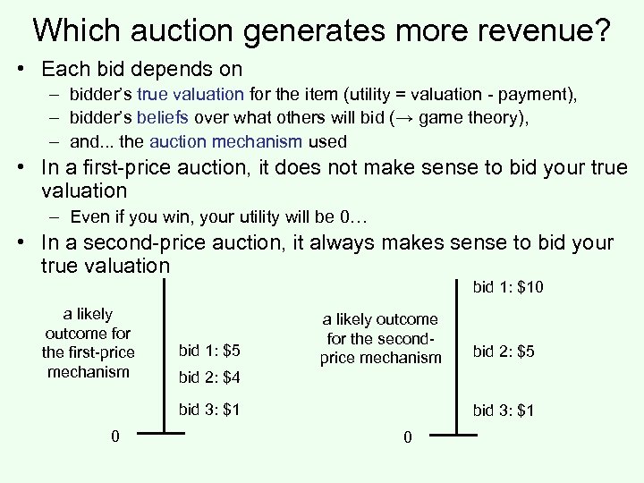Which auction generates more revenue? • Each bid depends on – bidder’s true valuation for the item (utility = valuation - payment), – bidder’s beliefs over what others will bid (→ game theory), – and. . . the auction mechanism used • In a first-price auction, it does not make sense to bid your true valuation – Even if you win, your utility will be 0… • In a second-price auction, it always makes sense to bid your true valuation bid 1: $10 a likely outcome for the first-price mechanism bid 1: $5 a likely outcome for the secondprice mechanism bid 2: $4 bid 3: $1 0 bid 2: $5 bid 3: $1 0

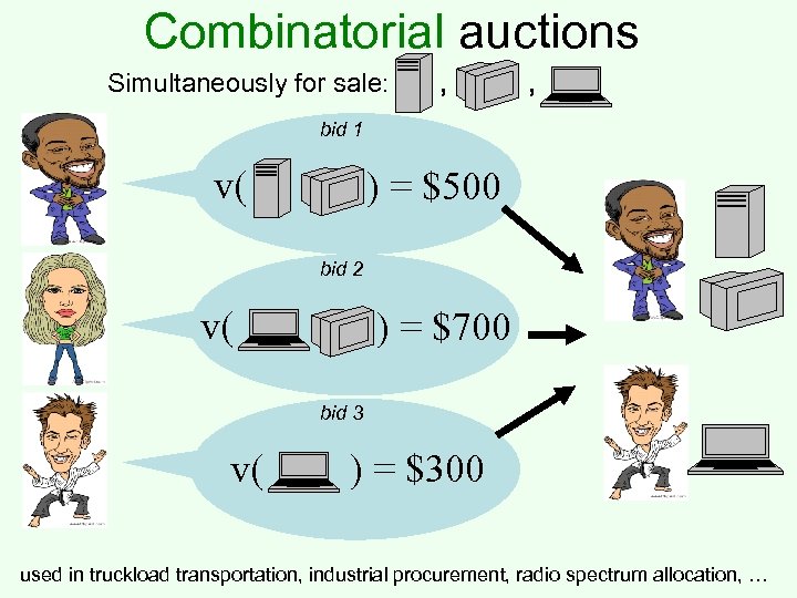Combinatorial auctions Simultaneously for sale: , , bid 1 v( ) = $500 bid 2 v( ) = $700 bid 3 v( ) = $300 used in truckload transportation, industrial procurement, radio spectrum allocation, …

Combinatorial auction problems • Winner determination problem – Deciding which bids win is (in general) a hard computational problem (NP-hard) • Preference elicitation (communication) problem – In general, each bidder may have a different value for each bundle – But it may be impractical to bid on every bundle (there are exponentially many bundles) • Mechanism design problem – How do we get the bidders to behave so that we get good outcomes? • These problems interact in nontrivial ways – E. g. limited computational or communication capacity limits mechanism design options

Risk attitudes • Which would you prefer? – A lottery ticket that pays out $10 with probability. 5 and $0 otherwise, or – A lottery ticket that pays out $3 with probability 1 • How about: – A lottery ticket that pays out $100, 000 with probability. 5 and $0 otherwise, or – A lottery ticket that pays out $30, 000 with probability 1 • Usually, people do not simply go by expected value • An agent is risk-neutral if she only cares about the expected value of the lottery ticket • An agent is risk-averse if she always prefers the expected value of the lottery ticket to the lottery ticket – Most people are like this • An agent is risk-seeking if she always prefers the lottery ticket to the expected value of the lottery ticket

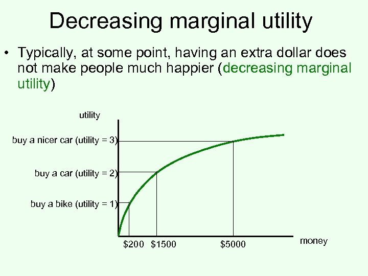Decreasing marginal utility • Typically, at some point, having an extra dollar does not make people much happier (decreasing marginal utility) utility buy a nicer car (utility = 3) buy a car (utility = 2) buy a bike (utility = 1) $200 $1500 $5000 money

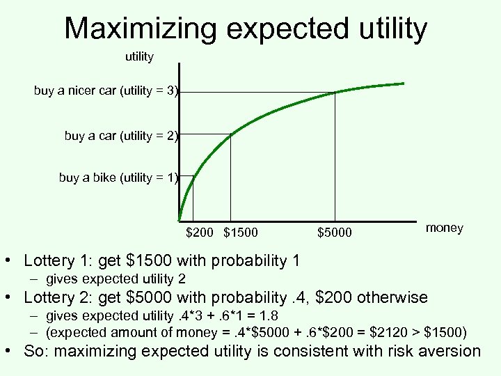Maximizing expected utility buy a nicer car (utility = 3) buy a car (utility = 2) buy a bike (utility = 1) $200 $1500 $5000 money • Lottery 1: get $1500 with probability 1 – gives expected utility 2 • Lottery 2: get $5000 with probability. 4, $200 otherwise – gives expected utility. 4*3 +. 6*1 = 1. 8 – (expected amount of money =. 4*$5000 +. 6*$200 = $2120 > $1500) • So: maximizing expected utility is consistent with risk aversion

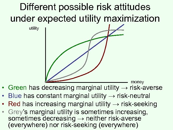Different possible risk attitudes under expected utility maximization utility • • money Green has decreasing marginal utility → risk-averse Blue has constant marginal utility → risk-neutral Red has increasing marginal utility → risk-seeking Grey’s marginal utility is sometimes increasing, sometimes decreasing → neither risk-averse (everywhere) nor risk-seeking (everywhere)

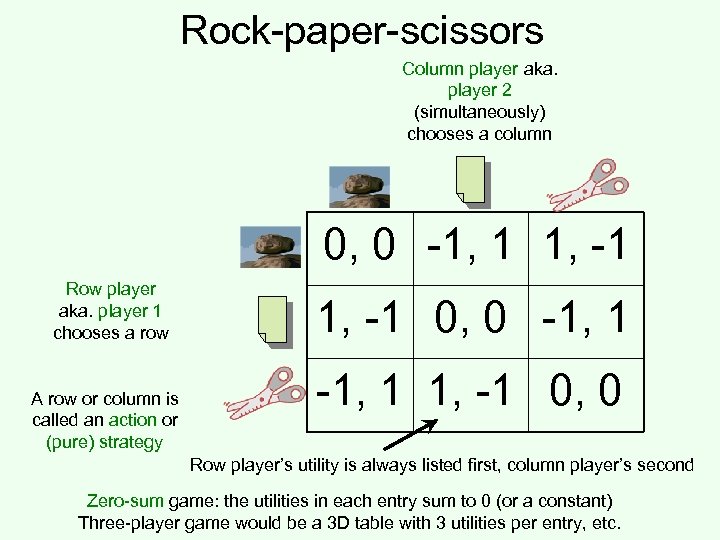Rock-paper-scissors Column player aka. player 2 (simultaneously) chooses a column 0, 0 -1, 1 1, -1 Row player aka. player 1 chooses a row A row or column is called an action or (pure) strategy 1, -1 0, 0 -1, 1 1, -1 0, 0 Row player’s utility is always listed first, column player’s second Zero-sum game: the utilities in each entry sum to 0 (or a constant) Three-player game would be a 3 D table with 3 utilities per entry, etc.

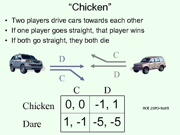“Chicken” • Two players drive cars towards each other • If one player goes straight, that player wins • If both go straight, they both die D C Chicken Dare D 0, 0 -1, 1 1, -1 -5, -5 not zero-sum

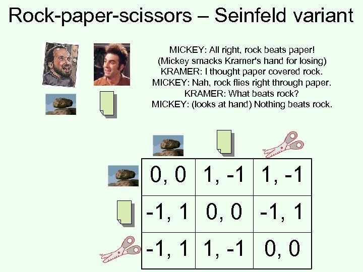Rock-paper-scissors – Seinfeld variant MICKEY: All right, rock beats paper! (Mickey smacks Kramer's hand for losing) KRAMER: I thought paper covered rock. MICKEY: Nah, rock flies right through paper. KRAMER: What beats rock? MICKEY: (looks at hand) Nothing beats rock. 0, 0 1, -1 -1, 1 0, 0 -1, 1 1, -1 0, 0

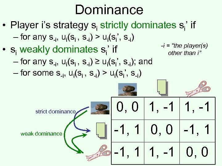Dominance • Player i’s strategy si strictly dominates si’ if – for any s-i, ui(si , s-i) > ui(si’, s-i) • si weakly dominates si’ if – for any s-i, ui(si , s-i) ≥ ui(si’, s-i); and – for some s-i, ui(si , s-i) > ui(si’, s-i) strict dominance weak dominance -i = “the player(s) other than i” 0, 0 1, -1 -1, 1 0, 0 -1, 1 1, -1 0, 0

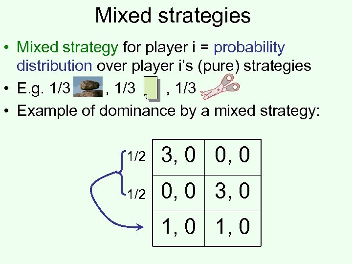Mixed strategies • Mixed strategy for player i = probability distribution over player i’s (pure) strategies • E. g. 1/3 , 1/3 • Example of dominance by a mixed strategy: 1/2 3, 0 0, 0 1/2 0, 0 3, 0 1, 0

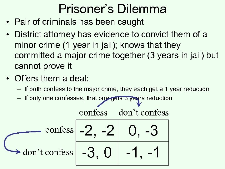Prisoner’s Dilemma • Pair of criminals has been caught • District attorney has evidence to convict them of a minor crime (1 year in jail); knows that they committed a major crime together (3 years in jail) but cannot prove it • Offers them a deal: – If both confess to the major crime, they each get a 1 year reduction – If only one confesses, that one gets 3 years reduction confess don’t confess -2, -2 0, -3 -3, 0 -1, -1

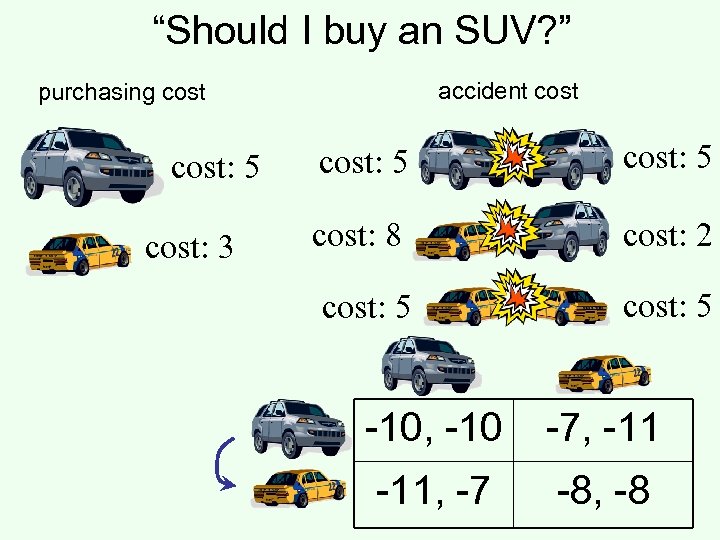“Should I buy an SUV? ” accident cost purchasing cost: 5 cost: 3 cost: 5 cost: 8 cost: 2 cost: 5 -10, -10 -7, -11, -7 -8, -8

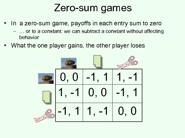Zero-sum games • In a zero-sum game, payoffs in each entry sum to zero – … or to a constant: we can subtract a constant without affecting behavior • What the one player gains, the other player loses 0, 0 -1, 1 1, -1 0, 0

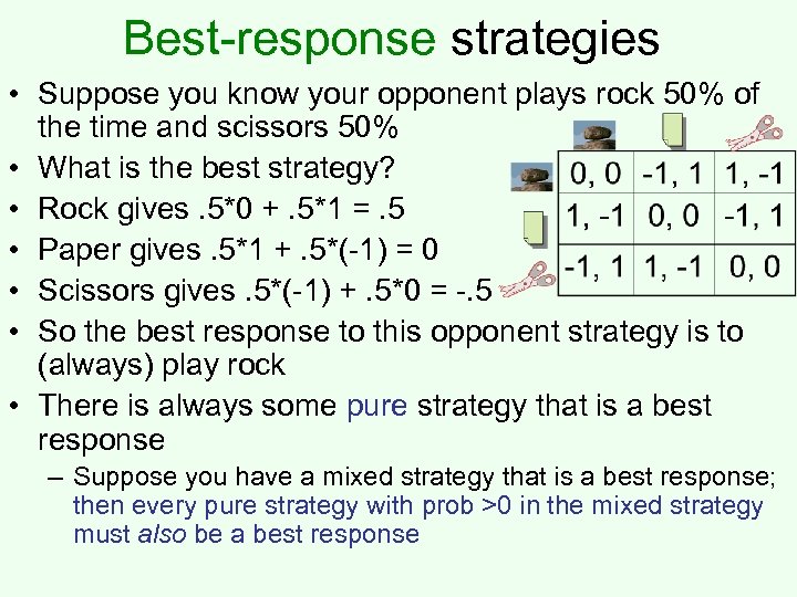Best-response strategies • Suppose you know your opponent plays rock 50% of the time and scissors 50% • What is the best strategy? • Rock gives. 5*0 +. 5*1 =. 5 • Paper gives. 5*1 +. 5*(-1) = 0 • Scissors gives. 5*(-1) +. 5*0 = -. 5 • So the best response to this opponent strategy is to (always) play rock • There is always some pure strategy that is a best response – Suppose you have a mixed strategy that is a best response; then every pure strategy with prob >0 in the mixed strategy must also be a best response

Minimax (minmax, maxmin) strategies • 2 -player zero-sum games: • Suppose that your opponent can see into your head and thus knows your mixed strategy • But does not know the random choices – E. g. your opponent knows that you play rock 50% of the time and scissors 50% of the time, but not which you will actually play – I. e. your opponent best-responds to your mixed strategy • What is the best that the row player can do against such a powerful column player? • maxσrow minscol urow(σrow, scol) – Here σrow is a mixed strategy, scol is a pure strategy, and utility functions are extended to mixed strategies by taking the expectation of the utility over pure strategies

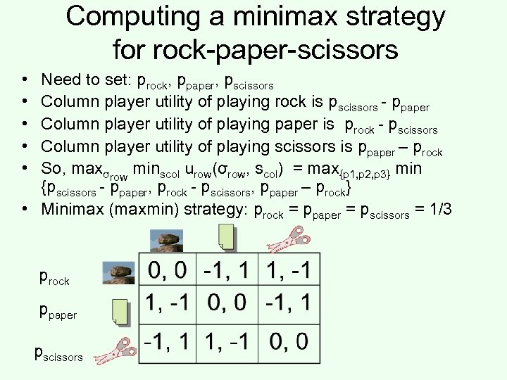Computing a minimax strategy for rock-paper-scissors • • • Need to set: prock, ppaper, pscissors Column player utility of playing rock is pscissors - ppaper Column player utility of playing paper is prock - pscissors Column player utility of playing scissors is ppaper – prock So, maxσrow minscol urow(σrow, scol) = max{p 1, p 2, p 3} min {pscissors - ppaper, prock - pscissors, ppaper – prock} • Minimax (maxmin) strategy: prock = ppaper = pscissors = 1/3 prock ppaper pscissors

Minimax theorem [von Neumann 1927] • In general, which one is bigger: – maxσrow minscol urow(σrow, scol) (col knows σrow), or – minσcol maxsrow urow(srow, σcol) (row knows σcol)? • Minimax Theorem: maxσrow minscol urow(σrow, scol) = minσcol maxsrow urow(srow, σcol) – This quantity is called the value of the game (to row player) • Follows from (predates) linear programming duality • Ergo: if you can look into the other player’s head (but the other player anticipates that), you will do no better than if the roles were reversed • Only true if we allow for mixed strategies – If you know the other player’s pure strategy in rock-paperscissors, you will always win

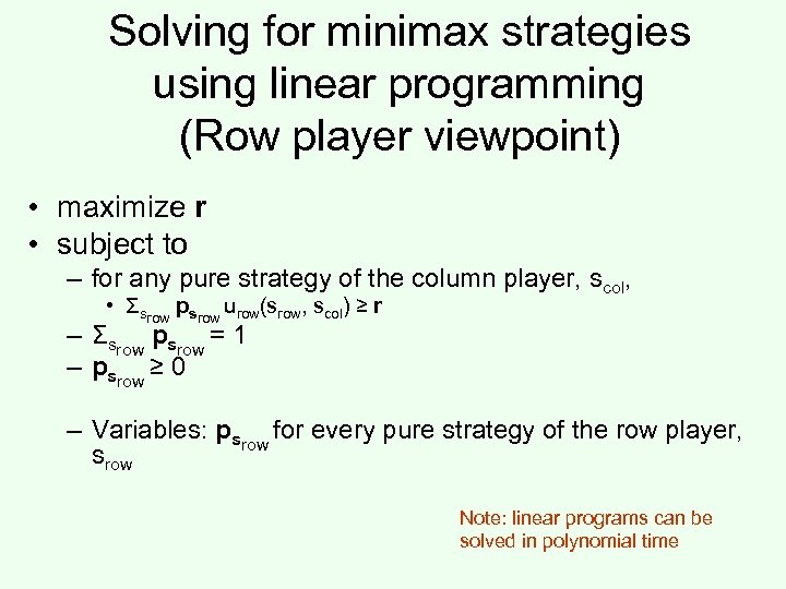Solving for minimax strategies using linear programming (Row player viewpoint) • maximize r • subject to – for any pure strategy of the column player, scol, • Σsrow psrow urow(srow, scol) ≥ r – Σsrow psrow = 1 – psrow ≥ 0 – Variables: psrow for every pure strategy of the row player, srow Note: linear programs can be solved in polynomial time

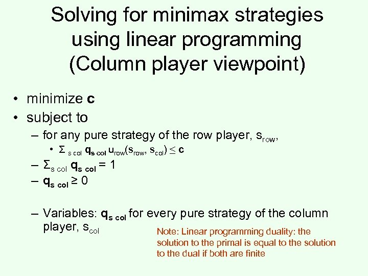Solving for minimax strategies using linear programming (Column player viewpoint) • minimize c • subject to – for any pure strategy of the row player, srow, • Σ s col qs col urow(srow, scol) ≤ c – Σs col qs col = 1 – qs col ≥ 0 – Variables: qs col for every pure strategy of the column player, scol Note: Linear programming duality: the solution to the primal is equal to the solution to the dual if both are finite

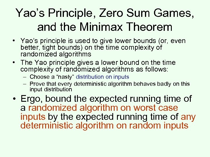Yao’s Principle, Zero Sum Games, and the Minimax Theorem • Yao’s principle is used to give lower bounds (or, even better, tight bounds) on the time complexity of randomized algorithms • The Yao principle gives a lower bound on the time complexity of randomized algorithms as follows: – Choose a “nasty” distribution on inputs – Prove that every deterministic algorithm behaves badly on this input distribution • Ergo, bound the expected running time of a randomized algorithm on worst case inputs by the expected running time of any deterministic algorithm on random inputs

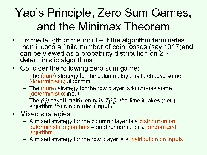Yao’s Principle, Zero Sum Games, and the Minimax Theorem • Fix the length of the input – if the algorithm terminates then it uses a finite number of coin tosses (say 1017)and can be viewed as a probability distribution on 21017 deterministic algorithms. • Consider the following zero sum game: – The (pure) strategy for the column player is to choose some (deterministic) algorithm – The (pure) strategy for the row player is to choose some (deterministic) input – The (i, j) payoff matrix entry is T(i, j): the time it takes (det. ) algorithm j to run on (det. ) input i • Mixed strategies: – A mixed strategy for the column player is a distribution on deterministic algorithms – another name for a randomized algorithm – A mixed strategy for the row player is a distribution on inputs.

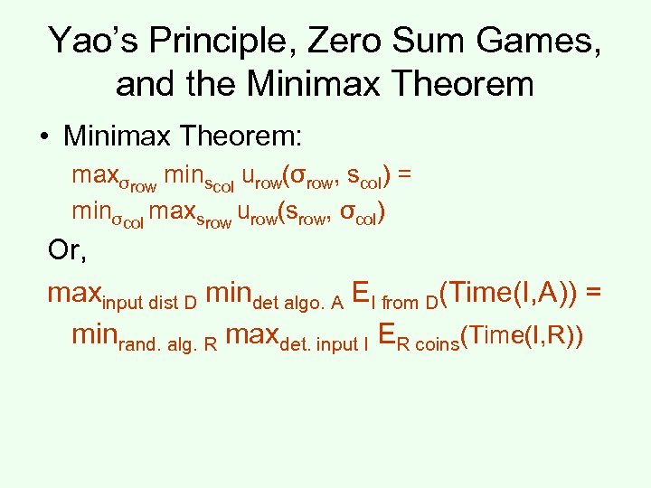Yao’s Principle, Zero Sum Games, and the Minimax Theorem • Minimax Theorem: maxσrow minscol urow(σrow, scol) = minσcol maxsrow urow(srow, σcol) Or, maxinput dist D mindet algo. A EI from D(Time(I, A)) = minrand. alg. R maxdet. input I ER coins(Time(I, R))

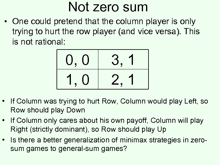Not zero sum • One could pretend that the column player is only trying to hurt the row player (and vice versa). This is not rational: 0, 0 1, 0 3, 1 2, 1 • If Column was trying to hurt Row, Column would play Left, so Row should play Down • If Column only cares about his own payoff, Column will play Right (strictly dominant), so Row should play Up • Is there a better generalization of minimax strategies in zerosum games to general-sum games?