Computational Game Theory Amos Fiat Spring 2012 Introduction

Computational Game Theory Amos Fiat Spring 2012 Introduction 1

Agenda Introduction to Game Theory Examples Matrix form Games Utility Solution concepts Dominant Strategies Nash Equilibria Complexity Mechanism Design: reverse game theory 2

Computational Game Theory The study of Game Theory in the context of Computer Science, in order to reason about problems from the perspective of computability and algorithm design. 3

CGT in Computer Science Computing involves many different selfish entities. Thus involves game theory. The Internet, Intranet, etc. ◦ Many players (end-users, ISVs, Infrastructure Providers) ◦ Players wish to maximize their own benefit and act accordingly ◦ The trick is to design a system where it’s beneficial for the player to follow the rules 4

CGT in Computer Science Theory ◦ Algorithm design ◦ Complexity ◦ Quality of game states (Equilibrium states in particular) ◦ Study of dynamics Industry ◦ Sponsored search ◦ Other auctions 5

Game Theory Rational Player ◦ Prioritizes possible actions according to utility or cost ◦ Strives to maximize utility or to minimize cost Competitive Environment ◦ More than one player at the same time Game Theory analyzes how rational players behave in competitive environments 6

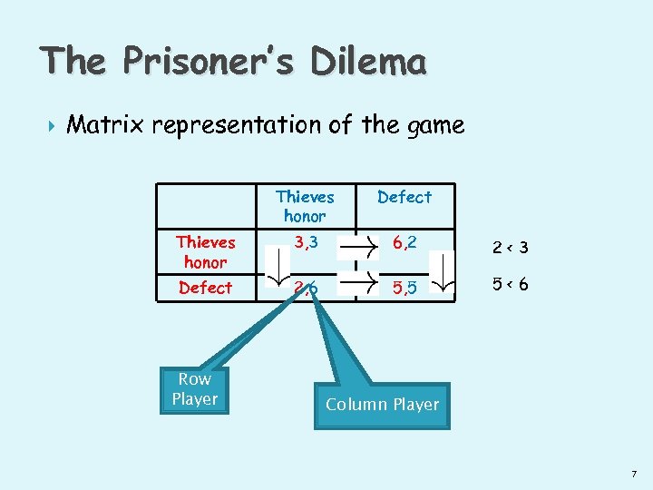The Prisoner’s Dilema Matrix representation of the game Thieves honor Defect Thieves honor 3, 3 6, 2 2<3 Defect 2, 6 5, 5 5<6 Row Player Column Player 7

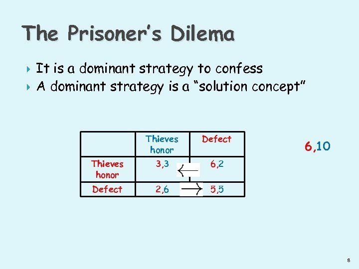The Prisoner’s Dilema It is a dominant strategy to confess A dominant strategy is a “solution concept” Thieves honor Defect Thieves honor 3, 3 6, 2 Defect 2, 6 5, 5 6, 10 8

ISP Routing Internet Service Providers (ISP) often share their physical networks for free In some cases an ISP can either choose to route traffic in its own network or via a partner network 9

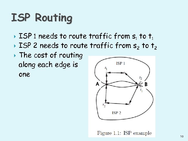ISP Routing ISP 1 needs to route traffic from s 1 to t 1 ISP 2 needs to route traffic from s 2 to t 2 The cost of routing along each edge is one A B 10

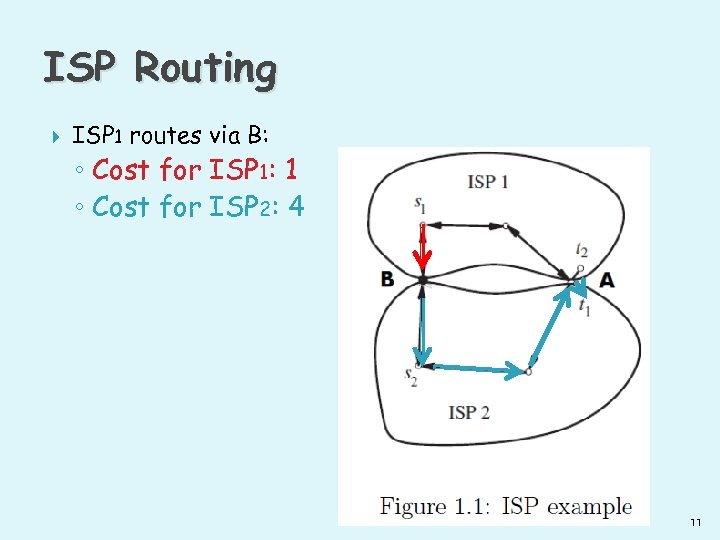ISP Routing ISP 1 routes via B: ◦ Cost for ISP 1: 1 ◦ Cost for ISP 2: 4 11

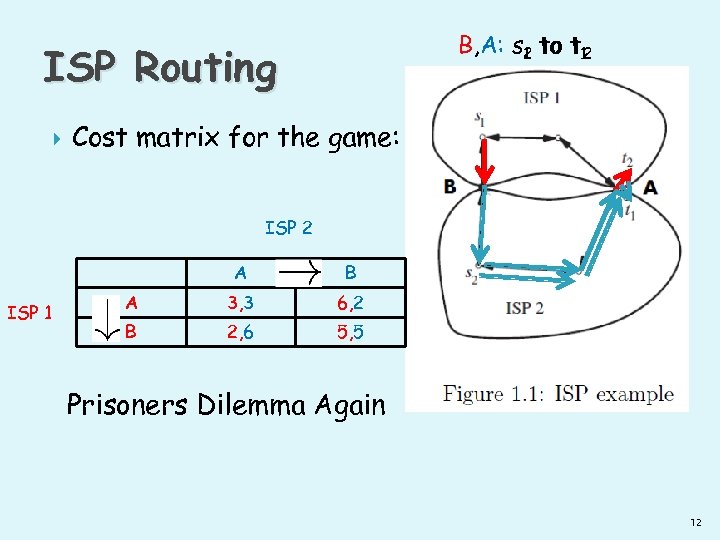B, A: s 1 to t 12 2 to t ISP Routing Cost matrix for the game: ISP 2 A ISP 1 B A 3, 3 6, 2 B 2, 6 5, 5 Prisoners Dilemma Again 12

Strategic Games The game consists of only one ‘turn’ All the players play simultaneously and are unaware of what the other players do Players are selfish, seek to maximize their own benefit 13

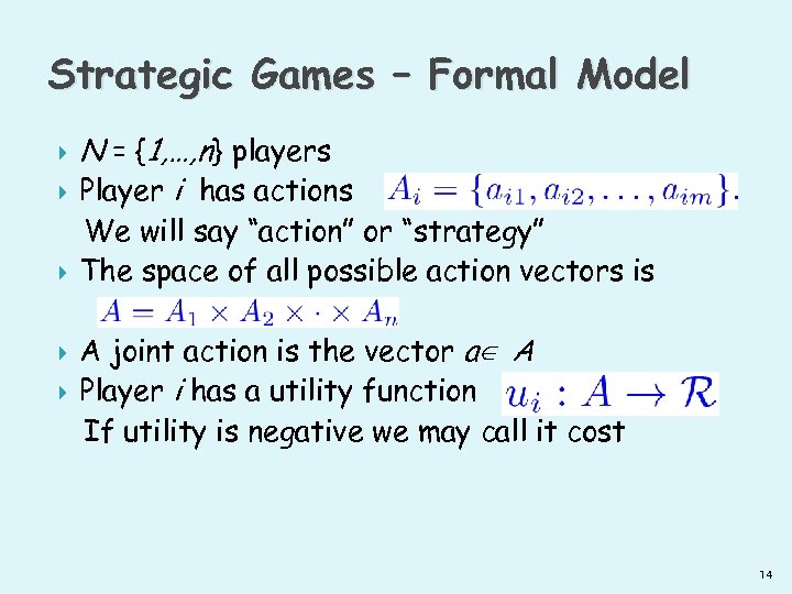Strategic Games – Formal Model N = {1, …, n} players Player i has actions We will say “action” or “strategy” The space of all possible action vectors is A joint action is the vector a∈ A Player i has a utility function If utility is negative we may call it cost 14

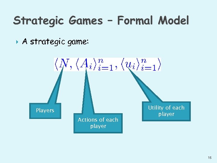Strategic Games – Formal Model A strategic game: Players Actions of each player Utility of each player 15

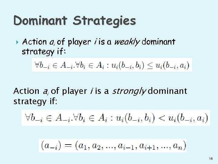Dominant Strategies Action ai of player i is a weakly dominant strategy if: Action ai of player i is a strongly dominant strategy if: 16

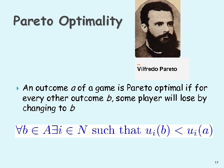Pareto Optimality Vilfredo Pareto An outcome a of a game is Pareto optimal if for every other outcome b, some player will lose by changing to b 17

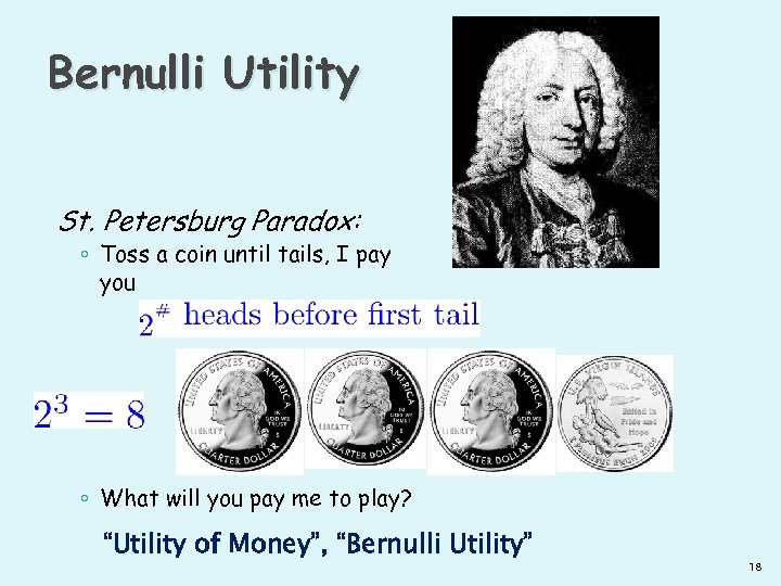Bernulli Utility St. Petersburg Paradox: ◦ Toss a coin until tails, I pay you ◦ What will you pay me to play? “Utility of Money”, “Bernulli Utility” 18

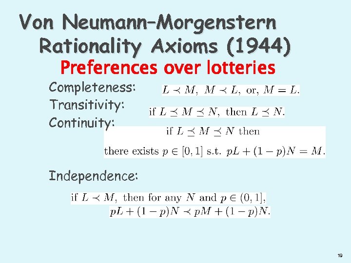Von Neumann–Morgenstern Rationality Axioms (1944) Preferences over lotteries Completeness: Transitivity: Continuity: Independence: 19

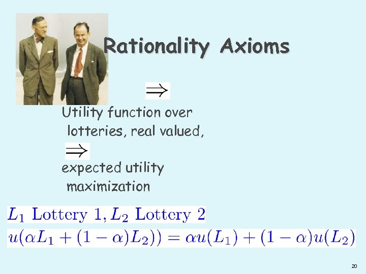Rationality Axioms Utility function over lotteries, real valued, expected utility maximization 20

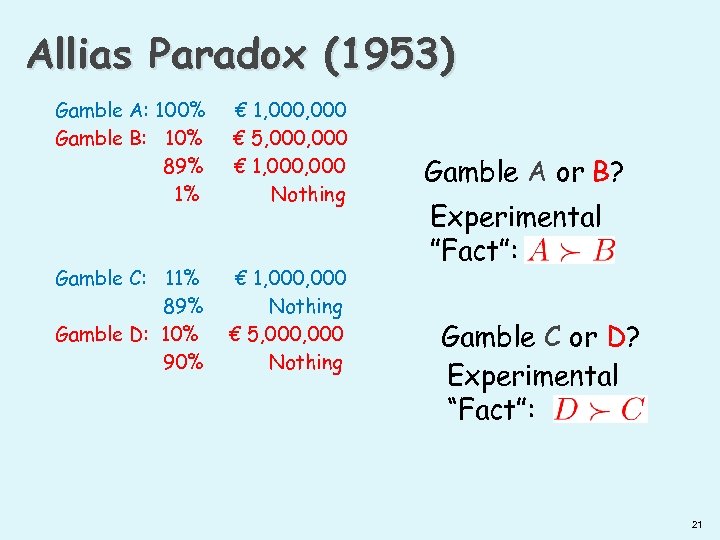Allias Paradox (1953) Gamble A: 100% Gamble B: 10% 89% 1% € 1, 000 € 5, 000 € 1, 000 Nothing Gamble C: 11% 89% Gamble D: 10% 90% € 1, 000 Nothing € 5, 000 Nothing Gamble A or B? Experimental ”Fact”: Gamble C or D? Experimental “Fact”: 21

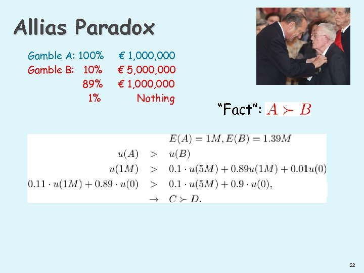Allias Paradox Gamble A: 100% Gamble B: 10% 89% 1% € 1, 000 € 5, 000 € 1, 000 Nothing Gamble C: 11% 89% Gamble D: 10% 90% € 1, 000 Nothing € 5, 000 Nothing “Fact”: 22

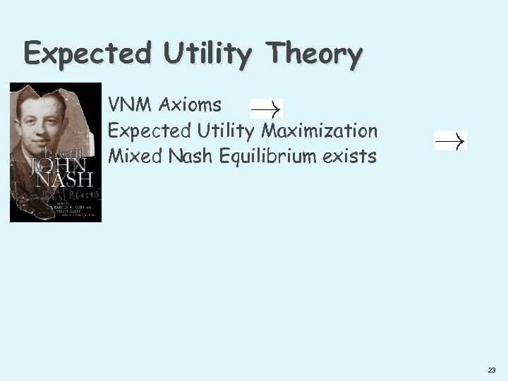Expected Utility Theory VNM Axioms Expected Utility Maximization Mixed Nash Equilibrium exists 23

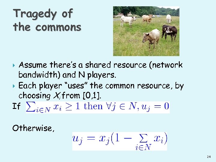Tragedy of the commons Assume there’s a shared resource (network bandwidth) and N players. Each player “uses” the common resource, by choosing Xi from [0, 1]. If Otherwise, 24

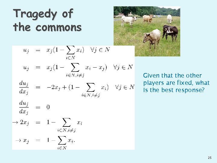Tragedy of the commons Given that the other players are fixed, what Is the best response? 25

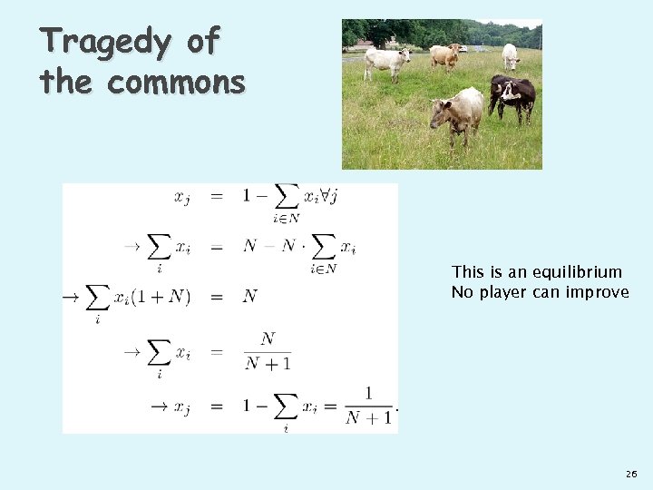Tragedy of the commons This is an equilibrium No player can improve 26

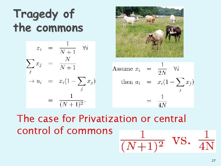Tragedy of the commons The case for Privatization or central control of commons 27

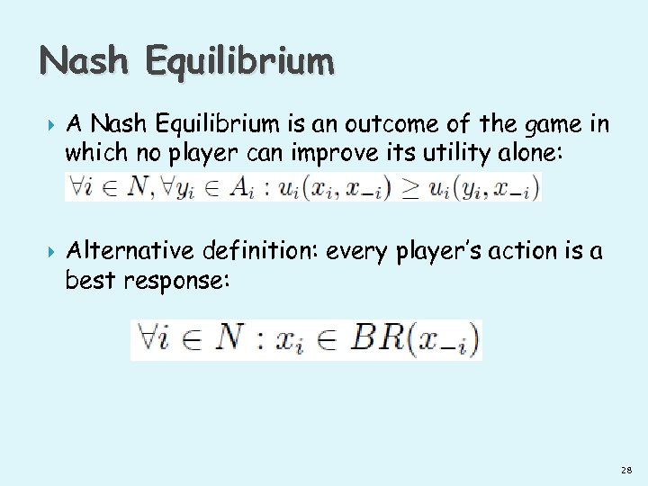Nash Equilibrium A Nash Equilibrium is an outcome of the game in which no player can improve its utility alone: Alternative definition: every player’s action is a best response: 28

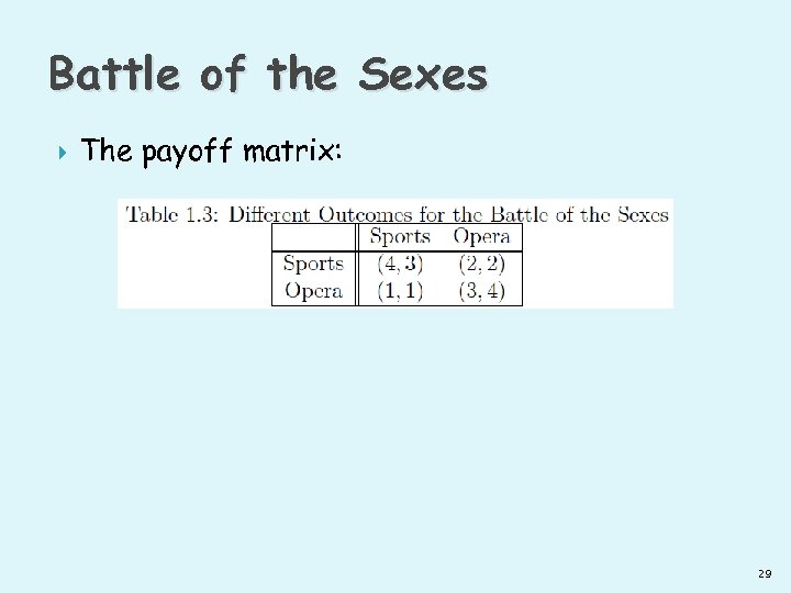Battle of the Sexes The payoff matrix: 29

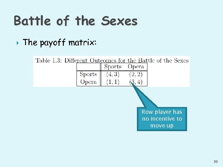Battle of the Sexes The payoff matrix: Row player has no incentive to move up 30

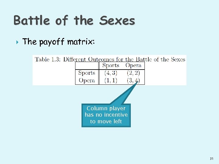Battle of the Sexes The payoff matrix: Column player has no incentive to move left 31

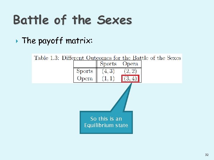Battle of the Sexes The payoff matrix: So this is an Equilibrium state 32

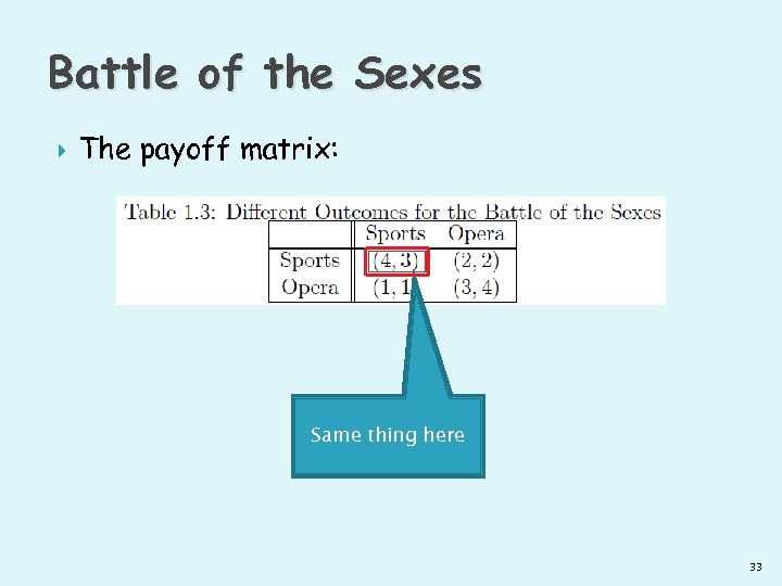Battle of the Sexes The payoff matrix: Same thing here 33

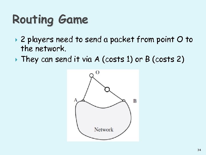Routing Game 2 players need to send a packet from point O to the network. They can send it via A (costs 1) or B (costs 2) 34

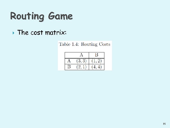Routing Game The cost matrix: 35

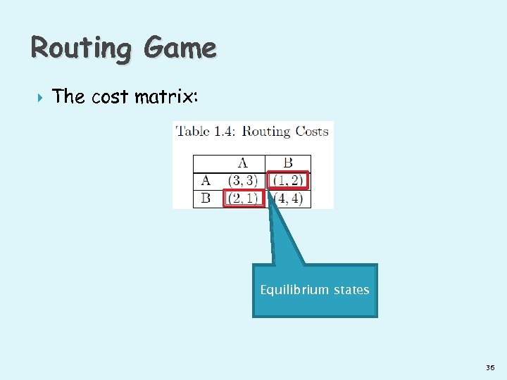Routing Game The cost matrix: Equilibrium states 36

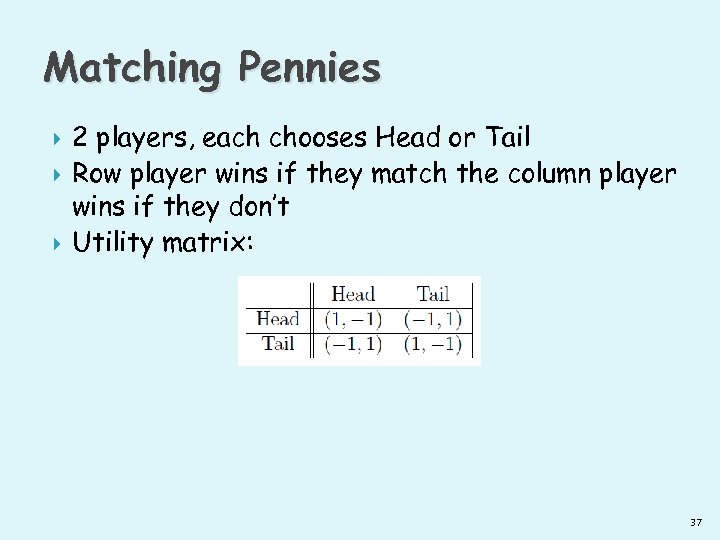Matching Pennies 2 players, each chooses Head or Tail Row player wins if they match the column player wins if they don’t Utility matrix: 37

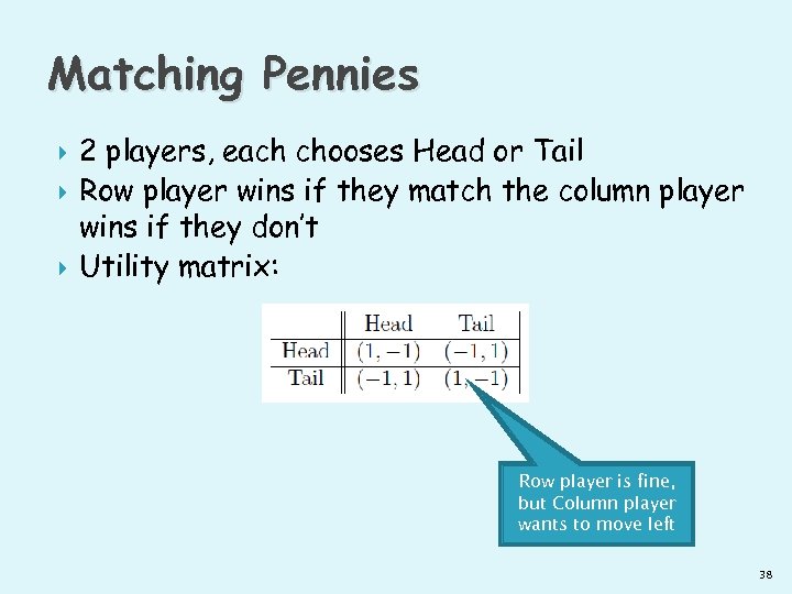Matching Pennies 2 players, each chooses Head or Tail Row player wins if they match the column player wins if they don’t Utility matrix: Row player is fine, but Column player wants to move left 38

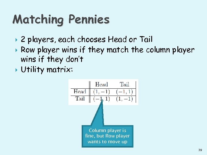Matching Pennies 2 players, each chooses Head or Tail Row player wins if they match the column player wins if they don’t Utility matrix: Column player is fine, but Row player wants to move up 39

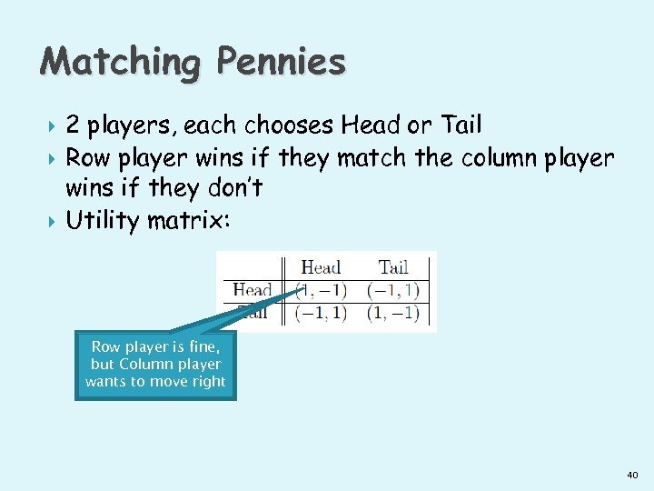Matching Pennies 2 players, each chooses Head or Tail Row player wins if they match the column player wins if they don’t Utility matrix: Row player is fine, but Column player wants to move right 40

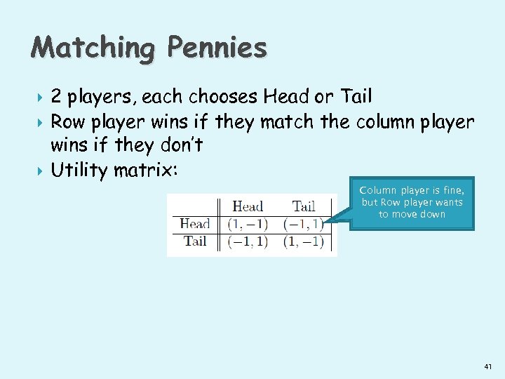Matching Pennies 2 players, each chooses Head or Tail Row player wins if they match the column player wins if they don’t Utility matrix: Column player is fine, but Row player wants to move down 41

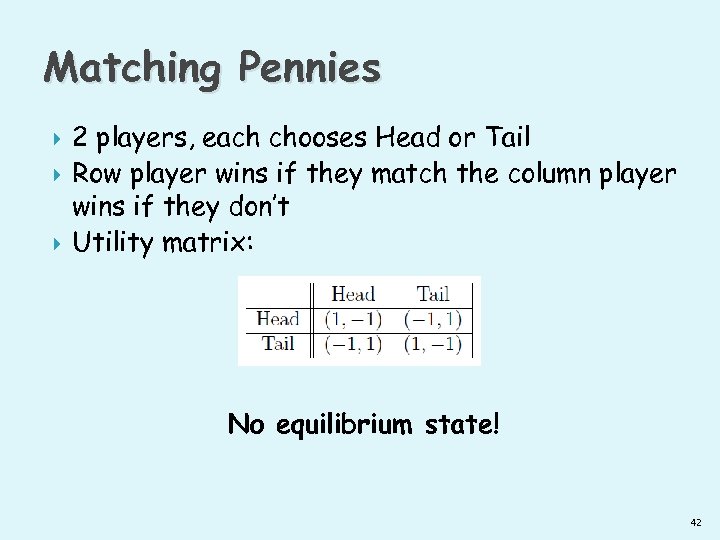Matching Pennies 2 players, each chooses Head or Tail Row player wins if they match the column player wins if they don’t Utility matrix: No equilibrium state! 42

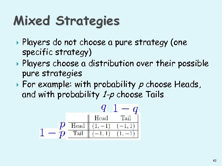Mixed Strategies Players do not choose a pure strategy (one specific strategy) Players choose a distribution over their possible pure strategies For example: with probability p choose Heads, and with probability 1 -p choose Tails 43

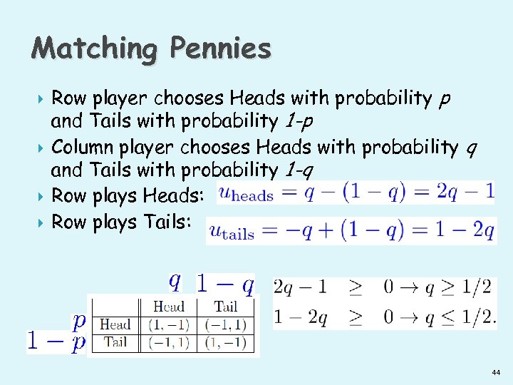Matching Pennies Row player chooses Heads with probability p and Tails with probability 1 -p Column player chooses Heads with probability q and Tails with probability 1 -q Row plays Heads: Row plays Tails: 44

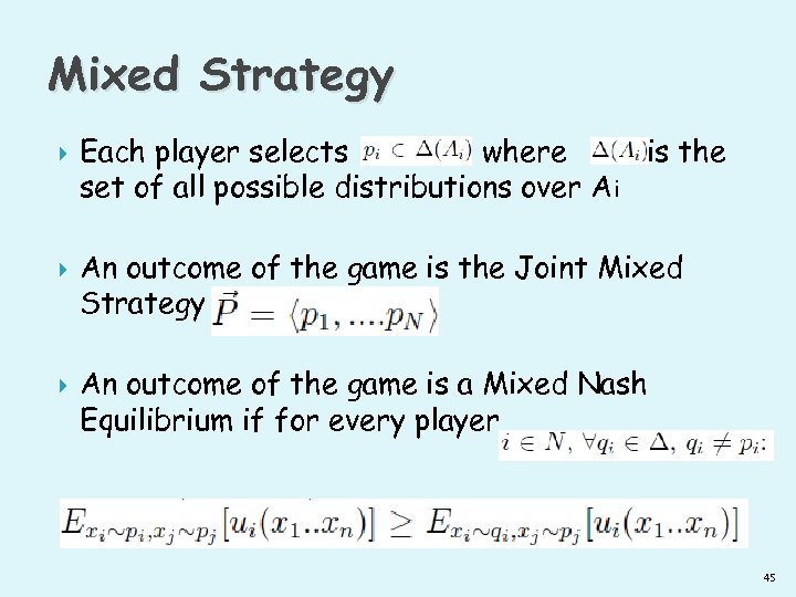Mixed Strategy Each player selects where is the set of all possible distributions over Ai An outcome of the game is the Joint Mixed Strategy An outcome of the game is a Mixed Nash Equilibrium if for every player 45

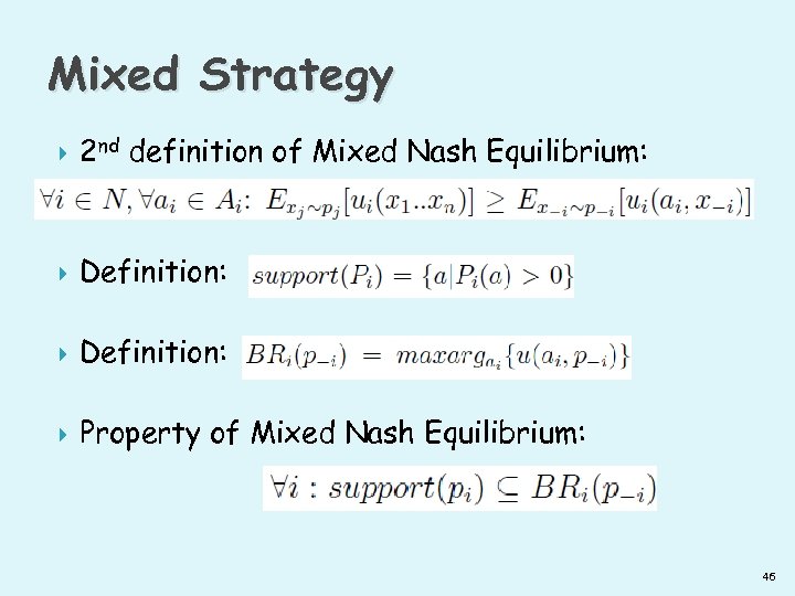Mixed Strategy 2 nd definition of Mixed Nash Equilibrium: Definition: Property of Mixed Nash Equilibrium: 46

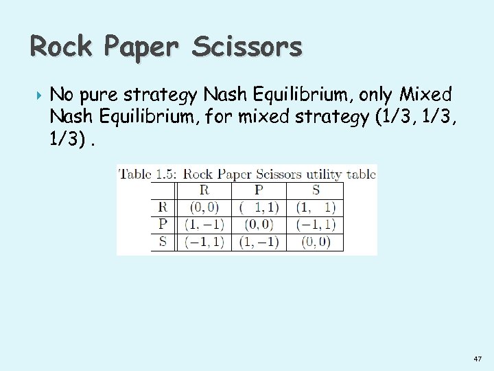Rock Paper Scissors No pure strategy Nash Equilibrium, only Mixed Nash Equilibrium, for mixed strategy (1/3, 1/3). 47

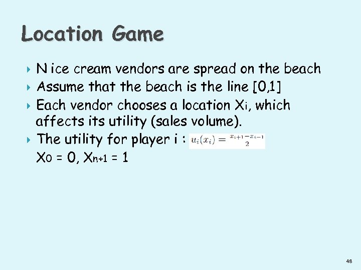Location Game N ice cream vendors are spread on the beach Assume that the beach is the line [0, 1] Each vendor chooses a location Xi, which affects its utility (sales volume). The utility for player i : X 0 = 0, Xn+1 = 1 48

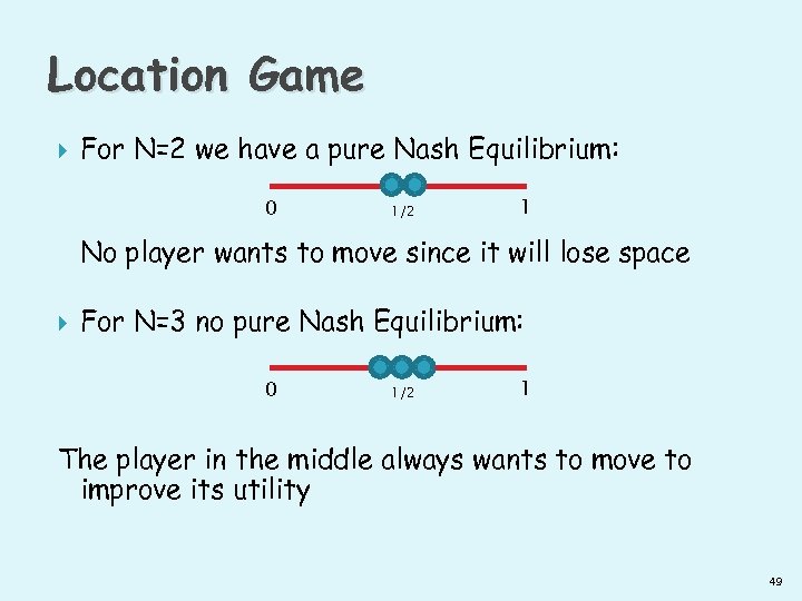Location Game For N=2 we have a pure Nash Equilibrium: 0 1/2 1 No player wants to move since it will lose space For N=3 no pure Nash Equilibrium: 0 1/2 1 The player in the middle always wants to move to improve its utility 49

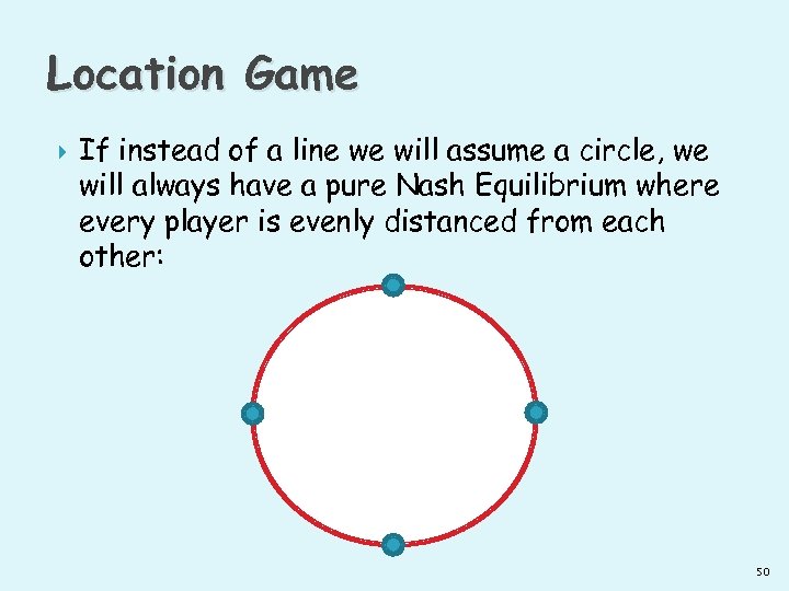Location Game If instead of a line we will assume a circle, we will always have a pure Nash Equilibrium where every player is evenly distanced from each other: 50

The Lemonade Stand Game http: //martin. zinkevich. org/lemonade/ http: //tech. groups. yahoo. com/group/lemonadeg ame/ 51

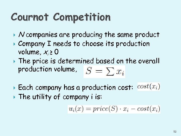Cournot Competition N companies are producing the same product Company I needs to choose its production volume, xi ≥ 0 The price is determined based on the overall production volume, Each company has a production cost: The utility of company i is: 52

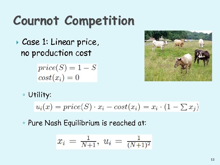Cournot Competition Case 1: Linear price, no production cost ◦ Utility: ◦ Pure Nash Equilibrium is reached at: 53

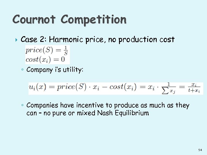Cournot Competition Case 2: Harmonic price, no production cost ◦ Company i’s utility: ◦ Companies have incentive to produce as much as they can – no pure or mixed Nash Equilibrium 54

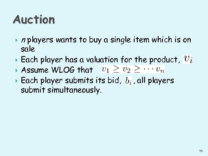Auction n players wants to buy a single item which is on sale Each player has a valuation for the product, Assume WLOG that Each player submits bid, , all players submit simultaneously. 55

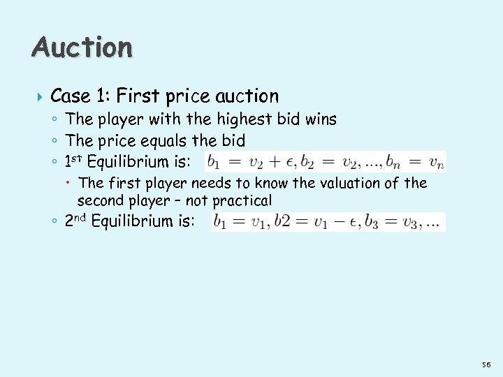Auction Case 1: First price auction ◦ The player with the highest bid wins ◦ The price equals the bid ◦ 1 st Equilibrium is: The first player needs to know the valuation of the second player – not practical ◦ 2 nd Equilibrium is: 56

Auction Case 2: Second price auction: Vickrey Auction ◦ The player with the highest bid wins ◦ The price equals the second highest bid No incentive to bid higher than one’s valuation - a player’s utility when it bids its valuation is at least as high than when it bids any other value This mechanism encourages players to bid truthfully Mechanism Design: reverse game theory – set up a game so that the equilibria has a desired property 57

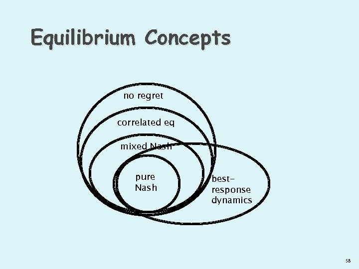Equilibrium Concepts no regret correlated eq mixed Nash pure Nash bestresponse dynamics 58

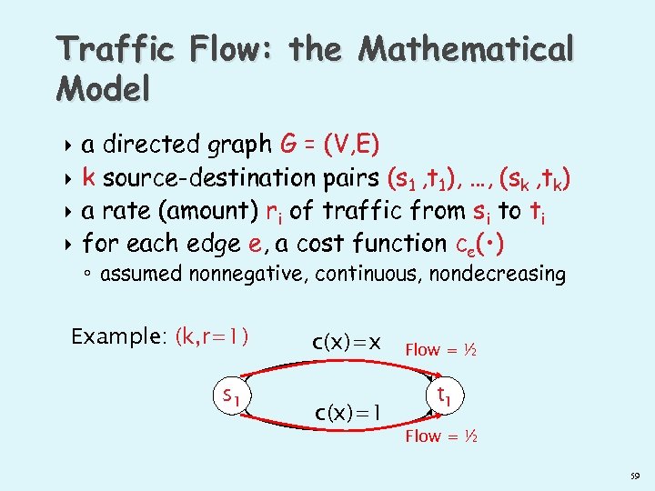Traffic Flow: the Mathematical Model a directed graph G = (V, E) k source-destination pairs (s 1 , t 1), …, (sk , tk) a rate (amount) ri of traffic from si to ti for each edge e, a cost function ce( • ) ◦ assumed nonnegative, continuous, nondecreasing Example: (k, r=1) s 1 c(x)=x c(x)=1 Flow = ½ t 1 Flow = ½ 59

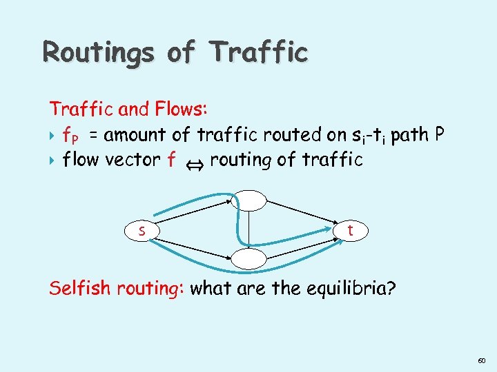Routings of Traffic and Flows: f. P = amount of traffic routed on si-ti path P flow vector f routing of traffic s t Selfish routing: what are the equilibria? 60

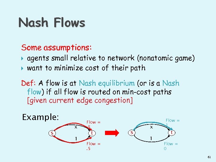Nash Flows Some assumptions: agents small relative to network (nonatomic game) want to minimize cost of their path Def: A flow is at Nash equilibrium (or is a Nash flow) if all flow is routed on min-cost paths [given current edge congestion] Example: s x 1 Flow =. 5 t Flow =. 5 s x 1 Flow = 1 t Flow = 0 61

History + Generalizations model, defn of Nash flows by [Wardrop 52] Nash flows exist, are (essentially) unique congestion game (payoffs fn of # of players) potential game (equilibria as optima) ◦ due to [Beckmann et al. 56] ◦ general nonatomic games: [Schmeidler 73] ◦ defined for atomic games by [Rosenthal 73] ◦ previous focus: Nash eq in pure strategies exist ◦ defined by [Monderer/Shapley 96] 62

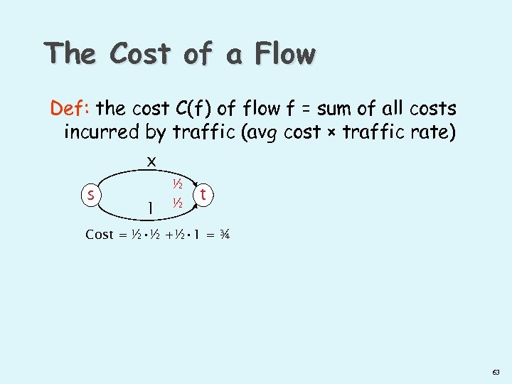The Cost of a Flow Def: the cost C(f) of flow f = sum of all costs incurred by traffic (avg cost × traffic rate) x s 1 ½ ½ t Cost = ½ • ½ +½ • 1 = ¾ 63

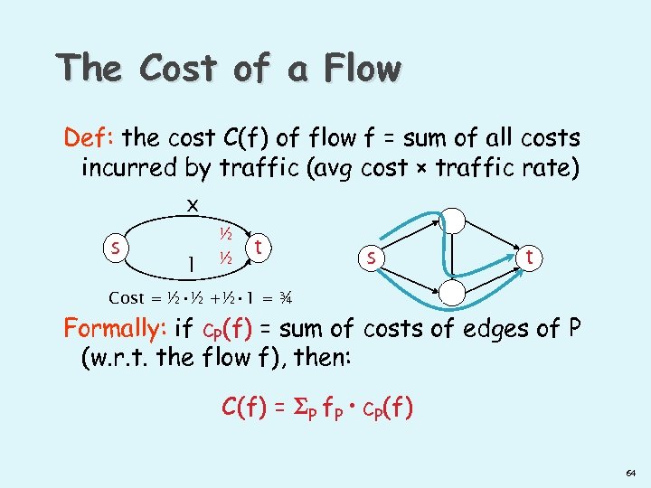The Cost of a Flow Def: the cost C(f) of flow f = sum of all costs incurred by traffic (avg cost × traffic rate) x s 1 ½ ½ t s t Cost = ½ • ½ +½ • 1 = ¾ Formally: if c. P(f) = sum of costs of edges of P (w. r. t. the flow f), then: C(f) = P f. P • c. P(f) 64

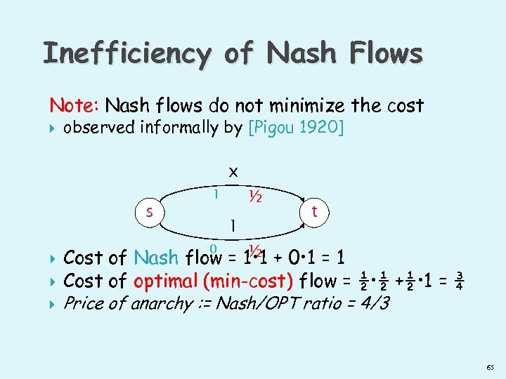Inefficiency of Nash Flows Note: Nash flows do not minimize the cost observed informally by [Pigou 1920] x s 1 1 ½ t ½ Cost of Nash flow = 1 • 1 + 0 • 1 = 1 Cost of optimal (min-cost) flow = ½ • ½ +½ • 1 = ¾ 0 Price of anarchy : = Nash/OPT ratio = 4/3 65

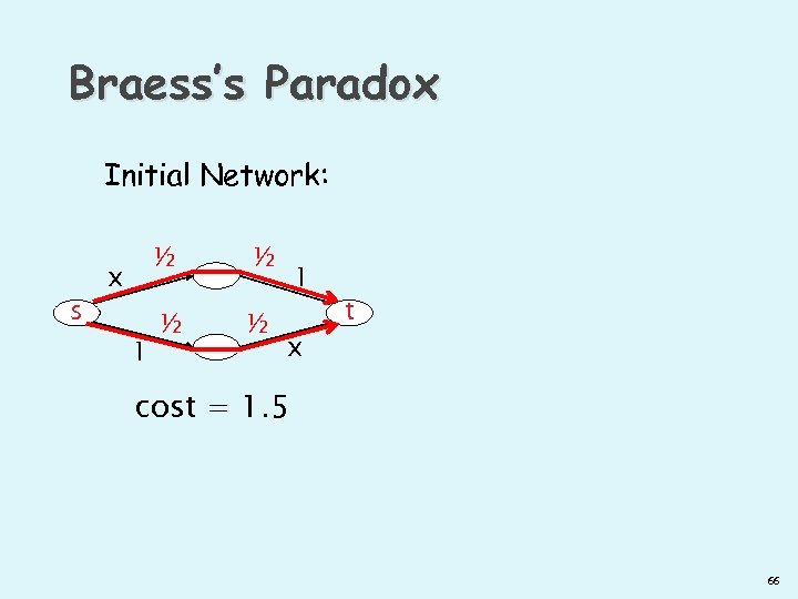Braess’s Paradox Initial Network: s ½ x 1 ½ ½ ½ 1 x t cost = 1. 5 66

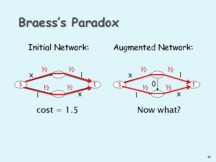Braess’s Paradox Initial Network: s ½ x 1 ½ ½ ½ 1 x cost = 1. 5 Augmented Network: t s ½ x 1 ½ ½ 0 ½ 1 x t Now what? 67

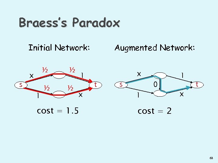Braess’s Paradox Initial Network: s ½ x 1 ½ ½ ½ 1 x cost = 1. 5 Augmented Network: t s x 1 0 1 x t cost = 2 68

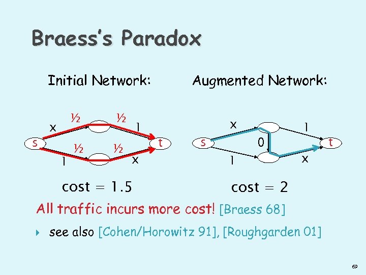Braess’s Paradox Initial Network: s ½ x 1 ½ ½ ½ 1 x cost = 1. 5 Augmented Network: t s x 1 0 1 x t cost = 2 All traffic incurs more cost! [Braess 68] see also [Cohen/Horowitz 91], [Roughgarden 01] 69