bf9a08a78a4d802da771364db7e8ae92.ppt
- Количество слайдов: 27
Computational Functional Genomics (26 -BE-790) (Statistical Models in Computational Biology) Instructor: Mario Medvedovic, Mario. Medvedovic@uc. edu Teaching Assistants: Johannes Freudenberg (Bioinformatics), Junhai Guo (Biostatistics), http: //eh 3. uc. edu/Computational. Functional. Genomics. html 1 -4 -2005 1

Course Outline • Everything will be posted on the web-site – • The course will start from very beginning in three different areas: – – – • • lecture slides, links to the papers to read, syllabus, computer programs, data, homework, etc Molecular genetics Statistics and probability Programming People with different backgrounds will need to focus their efforts differently Independent readings and practice is expected Access to a reasonably good PC computer with ability to install additional software is absolutely necessary The focus of the course is analysis of microarray data: experimental design, normalization, identification of differentially expressed genes, cluster analysis microarray data based classification, interpretation. Towards the end, statistical models for regulatory motifs will also be discussed If time permits, applications of general graphical models will also be discussed Getting to actual practical microarray data analysis very quickly – next lecture Filling in gaps as we go 1 -4 -2005 2
Course Outline • · · · · Basic concepts of molecular genetics, microarray technology, sources of variability, motivation of the need for statistical analysis Introduction to programming and data analysis using R and Bioconductor. Basics of probability theory (random events, probability, random variables, probability distributions, conditional probability) Basics of statistical inference (statistical models, random sample, parameter estimation, hypothesis testing, p-value) Identifying differentially expressed genes (normalization approaches, t-test, multiple comparison adjustments) Cluster analysis Functional clustering and identifying affected biological pathways Mid-term exam (in-class) Elements of Experimental design as applied to microarray data (Random block design, Confounding, Analysis of Variance, Elements of optimal design) Basics of Bayesian statistical inference (Bayes theorem, Hierarchical models, Empirical Bayes approaches for identifying differentially expressed genes) Statistical models in cluster analysis (hierarchical approaches, partitioning approaches, mixture model based clustering, EM algorithm, Gibbs sampling) Supervised machine learning and molecular fingerprinting using microarray data Statistical models and computational tools for identifying genomic regulatory elements Bayesian graphical models in functional genomics Final Project 1 -4 -2005 3
References No single universal reference textbook · A Primer of Genome Science. Gibson, G. , Muse, S. V. · Introductory Statistics with R. Peter Delgraad. Springer. Verlag, NY, 2002. · Bioinformatics and Computational Biology Solutions Using R and Bioconductor. Gentleman, R. , Carey, V. , Huber, W. , Irizarry, R. , Dudoit, S. Springer. · Bioinformatics: The machine learning approach/ Baldi, P. , Brunak, S. · Statistical methods in bioinformatics: an introduction / Warren J. Ewens, Gregory R. Grant 1 -4 -2005 4
Lecture Outline • • • Molecular genetics – “The Central Dogma” Functional Genomics – assigning function to genes Gene Expression – – – Functional Genomics Data – Microarrays Transcription and Regulatory motifs Computational Functional Genomics • • Stochasticity of functional genomics data and molecular biology in general – Measurement error • – – 1 -4 -2005 When measuring the same thing in the sample repeatedly “Biologic variability” • • Very wide area Computational analysis of functional genomics data Computational methods just a “front” of underlying statistical methods When measuring the same thing in multiple samples Stochasticity of underlying molecular processes Results in “noisy” data with significant stochastic components (microarray data, transcription factor binding motifs, protein folds, etc) 5
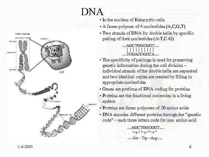
DNA • In the nucleus of Eukaryotic cells • A linear polymer of 4 nucleotides (A, C, G, T) • Two strands of DNA for double helix by specific pairing of their nucleotides (A-T, C-G) …AGCTGGCGGT… …TCGACCGCCA… • The specificity of pairings is used for preserving genetic information during the cell division – individual strands of the double helix are separated and two identical copies are created by filling in appropriate nucleotides • Genes are portions of DNA coding for proteins • Proteins are the functional molecules in a living system • Proteins are linear polymers of 20 amino acids • DNA encodes different proteins through the “genetic code” – each three letters code for one amino acid …AGCTGGCGGT… …-Ser - Trp –Arg-… 1 -4 -2005 6
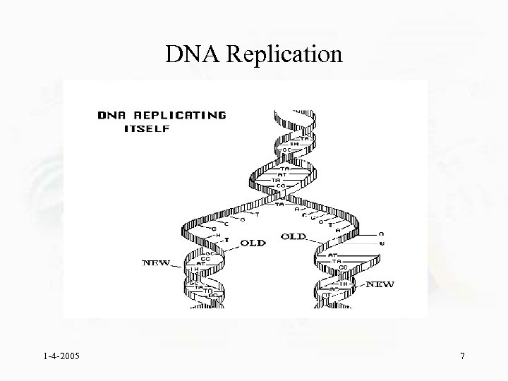
DNA Replication 1 -4 -2005 7
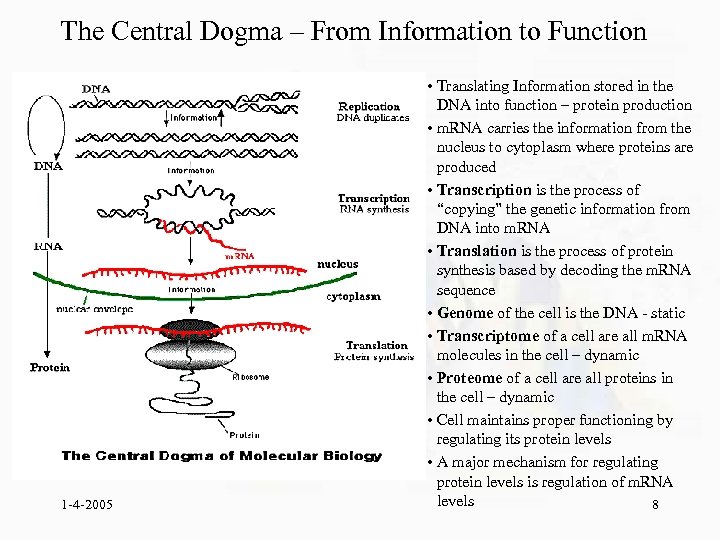
The Central Dogma – From Information to Function 1 -4 -2005 • Translating Information stored in the DNA into function – protein production • m. RNA carries the information from the nucleus to cytoplasm where proteins are produced • Transcription is the process of “copying” the genetic information from DNA into m. RNA • Translation is the process of protein synthesis based by decoding the m. RNA sequence • Genome of the cell is the DNA - static • Transcriptome of a cell are all m. RNA molecules in the cell – dynamic • Proteome of a cell are all proteins in the cell – dynamic • Cell maintains proper functioning by regulating its protein levels • A major mechanism for regulating protein levels is regulation of m. RNA levels 8
Functional Genomics • n : the branch of genomics that determines the biological function of the genes and their products – Source: Word. Net ® 2. 0, © 2003 Princeton University • Functional genomics data – Data that facilitates assigning function to genes or is directly assessing gene function (DNA/Protein sequence, 3 D protein structure, m. RNA levels measurements, etc. ) • Computational functional genomics (as assumed in this course) – Computational methods that facilitate application of appropriate mathematical/statistical models for analysis and interpretation of functional genomics data – In a broader sense, computational approaches to functional genomics 1 -4 -2005 9
Reading Materials Online Reading (in the suggested order): • An Introduction to biocomputing • Kimball’s Biology Pages – an online hypertext “textbook” – http: //www. techfak. uni-bielefeld. de/bcd/Curric/Introd/ch 0. html – http: //users. rcn. com/jkimball. ma. ultranet/Biology. Pages/T/Transcription. html – http: //users. rcn. com/jkimball. ma. ultranet/Biology. Pages/T/Translation. html Traditional References • • Lodish, H. et al. Molecular Cell Biology. (Ch 1), Ch 2, (Ch 3), Ch 4 Lewin, B. Genes. Ch 1 -Ch 3 Courses to Take • Introduction to Molecular Genetics 1 -4 -2005 10
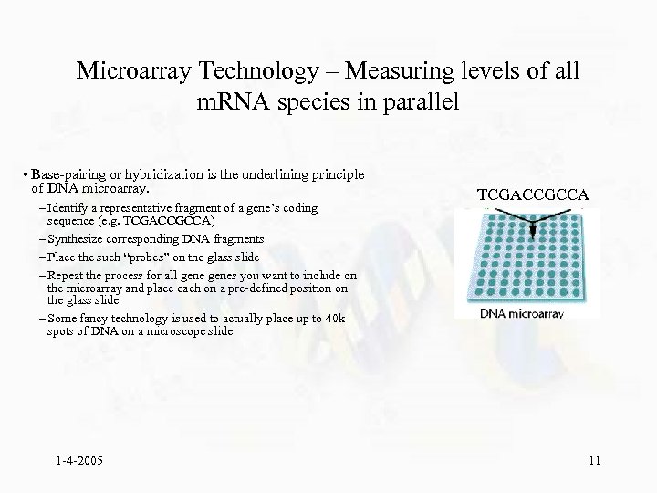
Microarray Technology – Measuring levels of all m. RNA species in parallel • Base-pairing or hybridization is the underlining principle of DNA microarray. – Identify a representative fragment of a gene’s coding sequence (e. g. TCGACCGCCA) – Synthesize corresponding DNA fragments – Place the such “probes” on the glass slide – Repeat the process for all genes you want to include on the microarray and place each on a pre-defined position on the glass slide – Some fancy technology is used to actually place up to 40 k spots of DNA on a microscope slide 1 -4 -2005 TCGACCGCCA 11
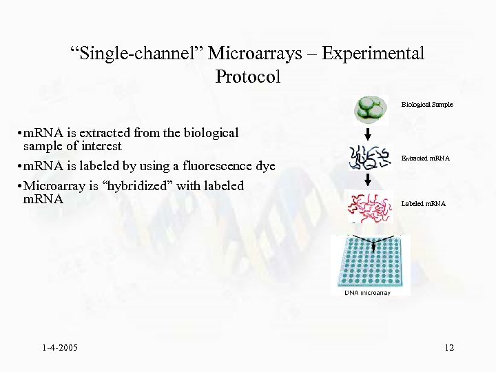
“Single-channel” Microarrays – Experimental Protocol Biological Sample • m. RNA is extracted from the biological sample of interest • m. RNA is labeled by using a fluorescence dye • Microarray is “hybridized” with labeled m. RNA 1 -4 -2005 Extracted m. RNA Labeled m. RNA 12
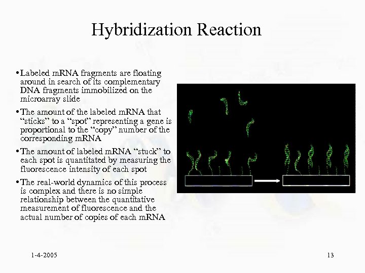
Hybridization Reaction • Labeled m. RNA fragments are floating around in search of its complementary DNA fragments immobilized on the microarray slide • The amount of the labeled m. RNA that “sticks” to a “spot” representing a gene is proportional to the “copy” number of the corresponding m. RNA • The amount of labeled m. RNA “stuck” to each spot is quantitated by measuring the fluorescence intensity of each spot • The real-world dynamics of this process is complex and there is no simple relationship between the quantitative measurement of fluorescence and the actual number of copies of each m. RNA 1 -4 -2005 13
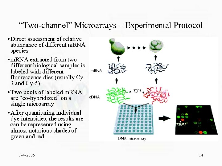
“Two-channel” Microarrays – Experimental Protocol • Direct assessment of relative abundance of different m. RNA species • m. RNA extracted from two different biological samples is labeled with different fluorescence dies (usually Cy 3 and Cy-5) • Two pools of labeled m. RNA are “co-hybridized” on a single microarray • After quantitating individual dye intensities, the results are can be represented using almost notorious shades of green and red 1 -4 -2005 14
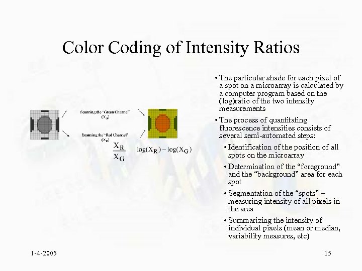
Color Coding of Intensity Ratios • The particular shade for each pixel of a spot on a microarray is calculated by a computer program based on the (log)ratio of the two intensity measurements • The process of quantitating fluorescence intensities consists of several semi-automated steps: • Identification of the position of all spots on the microarray • Determination of the “foreground” and the “background” area for each spot • Segmentation of the “spots” – measuring intensity of all pixels in the area • Summarizing the intensity of individual pixels (mean or median, variability measures, etc) 1 -4 -2005 15
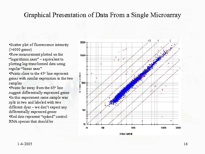
Graphical Presentation of Data From a Single Microarray • Scatter plot of fluorescence intensity (>6000 genes) • Row measurement plotted on the “logarithmic axes” – equivalent to plotting log-transformed data using regular “linear axes” • Points close to the 45 o line represent genes with similar expression in the two samples • Points far away from the 45 o line suggest differentially expressed genes • In this experiment same sample was split in two and labeled with two different dyes – we don’t expect any differentially expressed genes • Red dots represent “spiked” control RNA species that should be 1 -4 -2005 16
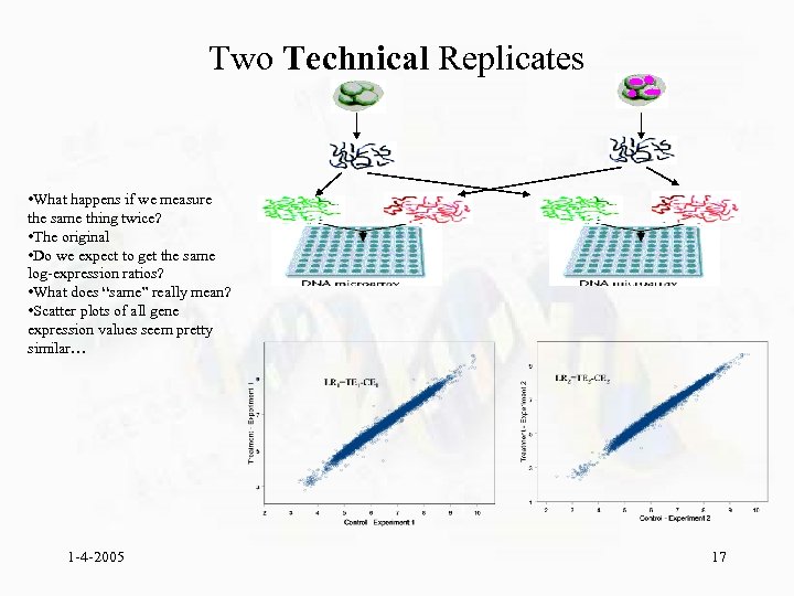
Two Technical Replicates • What happens if we measure the same thing twice? • The original • Do we expect to get the same log-expression ratios? • What does “same” really mean? • Scatter plots of all gene expression values seem pretty similar… 1 -4 -2005 17
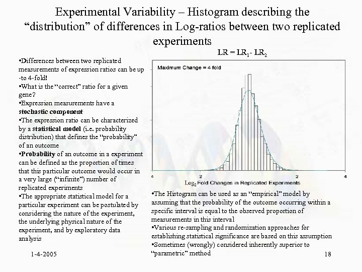
Experimental Variability – Histogram describing the “distribution” of differences in Log-ratios between two replicated experiments • Differences between two replicated measurements of expression ratios can be up -to 4 -fold! • What is the “correct” ratio for a given gene? • Expression measurements have a stochastic component • The expression ratio can be characterized by a statistical model (i. e. probability distribution) that defines the “probability” of an outcome • Probability of an outcome in a experiment can be defined as the proportion of times that this particular outcome would occur in a very large (“infinite”) number of replicated experiments • The appropriate statistical model for a particular experiment can be postulated by considering the nature of the experiment, the underlying physical nature of the experiment, and by exploratory data analysis 1 -4 -2005 LR = LR 1 - LR 2 • The Histogram can be used as an “empirical” model by assuming that the probability of the outcome occurring within a specific interval is equal to the observed proportion of measurements in this interval • Various re-sampling and randomization approaches for establishing statistical significance are based on this assumption • Sometimes (wrongly) considered inherently superior to “parametric” method 18
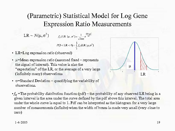
(Parametric) Statistical Model for Log Gene Expression Ratio Measurements • LR=Log expression ratio (observed) • =Mean expression ratio (assumed fixed – represents the signal of interest). This value is also the “expectation” of the LR, or the average of a very large (infinitely many) observations • =Standard Deviation – quantifying the variability of observations. • f. N =The probability distribution function (pdf) – the probability of any observed LR being in a given interval is the area under the curve defined by the pdf above this interval. The total area under the whole curve is equal to 1. Pdf can be interpreted as the histogram for a very large number of measurements (infinite) when the width of boxes is made very small (very close to zero) 1 -4 -2005 19
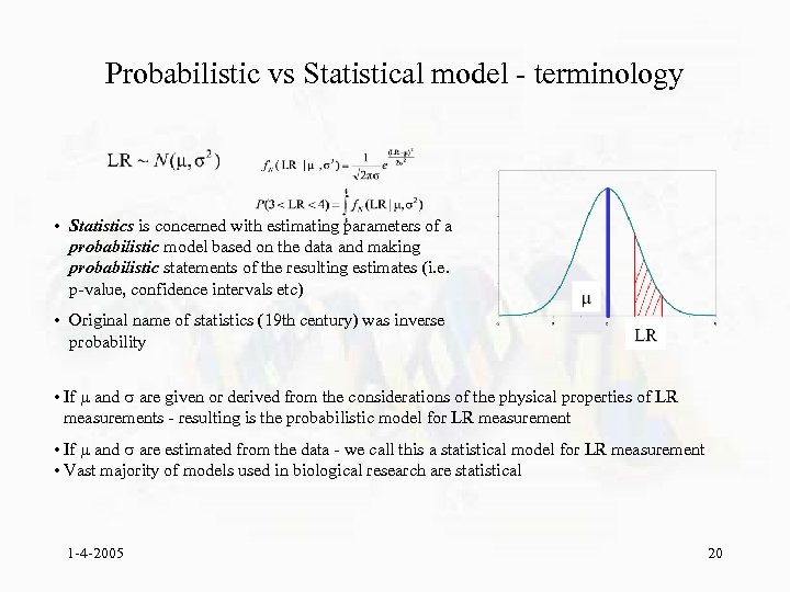
Probabilistic vs Statistical model - terminology • Statistics is concerned with estimating parameters of a probabilistic model based on the data and making probabilistic statements of the resulting estimates (i. e. p-value, confidence intervals etc) • Original name of statistics (19 th century) was inverse probability • If and are given or derived from the considerations of the physical properties of LR measurements - resulting is the probabilistic model for LR measurement • If and are estimated from the data - we call this a statistical model for LR measurement • Vast majority of models used in biological research are statistical 1 -4 -2005 20
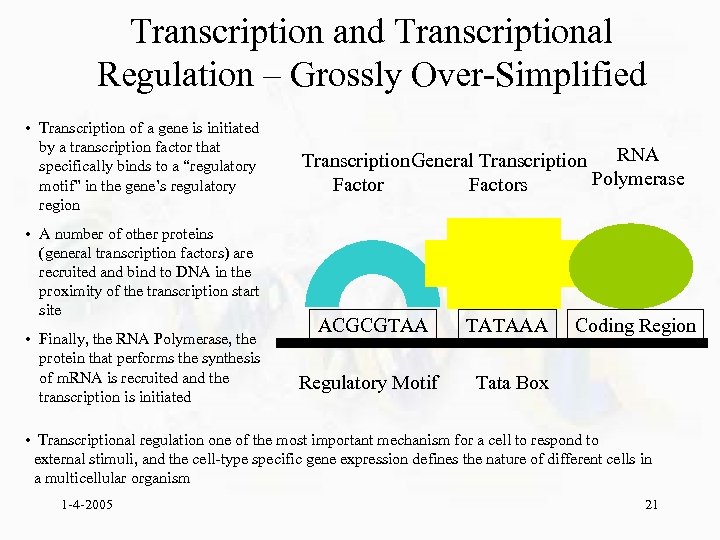
Transcription and Transcriptional Regulation – Grossly Over-Simplified • Transcription of a gene is initiated by a transcription factor that specifically binds to a “regulatory motif” in the gene’s regulatory region • A number of other proteins (general transcription factors) are recruited and bind to DNA in the proximity of the transcription start site • Finally, the RNA Polymerase, the protein that performs the synthesis of m. RNA is recruited and the transcription is initiated RNA Transcription General Transcription Polymerase Factors ACGCGTAA TATAAA Regulatory Motif Coding Region Tata Box • Transcriptional regulation one of the most important mechanism for a cell to respond to external stimuli, and the cell-type specific gene expression defines the nature of different cells in a multicellular organism 1 -4 -2005 21
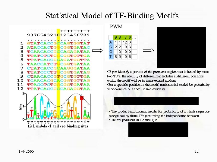
Statistical Model of TF-Binding Motifs • If you identify a portion of the promoter region that is bound by these two TF’s, the identity of different nucleotides at different positions within the motif will be to some extend random • For a specific position in the motif, multinomial model for probability of occurrence of a specific nucleotide is: • The product-multinomial model for probability of a whole sequence recognized by these TFs (assuming the independence between different positions in the motif) is: 1 -4 -2005 22
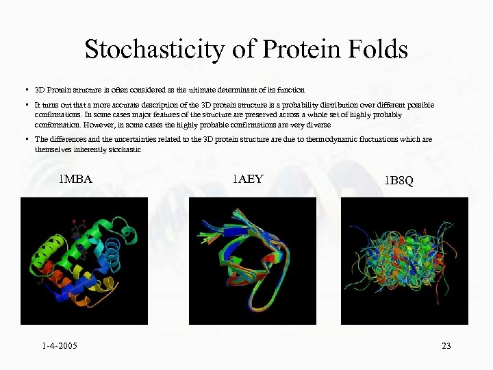
Stochasticity of Protein Folds • 3 D Protein structure is often considered as the ultimate determinant of its function • It turns out that a more accurate description of the 3 D protein structure is a probability distribution over different possible confirmations. In some cases major features of the structure are preserved across a whole set of highly probably conformation. However, in some cases the highly probable confirmations are very diverse • The differences and the uncertainties related to the 3 D protein structure are due to thermodynamic fluctuations which are themselves inherently stochastic 1 MBA 1 -4 -2005 1 AEY 1 B 8 Q 23
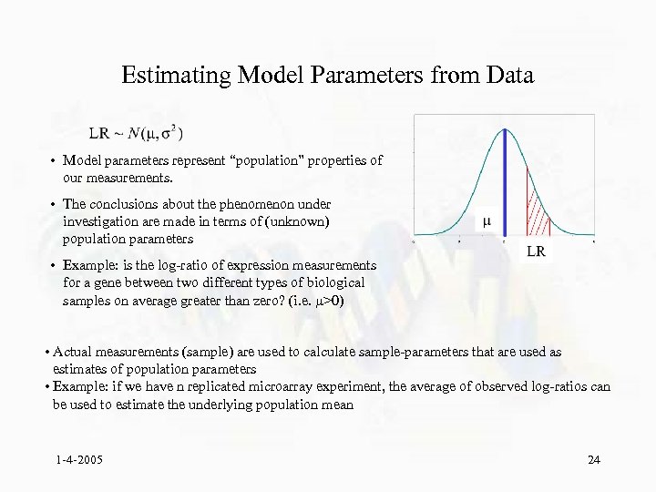
Estimating Model Parameters from Data • Model parameters represent “population” properties of our measurements. • The conclusions about the phenomenon under investigation are made in terms of (unknown) population parameters • Example: is the log-ratio of expression measurements for a gene between two different types of biological samples on average greater than zero? (i. e. >0) • Actual measurements (sample) are used to calculate sample-parameters that are used as estimates of population parameters • Example: if we have n replicated microarray experiment, the average of observed log-ratios can be used to estimate the underlying population mean 1 -4 -2005 24
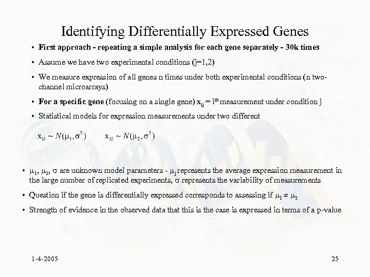
Identifying Differentially Expressed Genes • First approach - repeating a simple analysis for each gene separately - 30 k times • Assume we have two experimental conditions (j=1, 2) • We measure expression of all genes n times under both experimental conditions (n twochannel microarrays) • For a specific gene (focusing on a single gene) xij = ith measurement under condition j • Statistical models for expression measurements under two different • 1, 2, are unknown model parameters - j represents the average expression measurement in the large number of replicated experiments, represents the variability of measurements • Question if the gene is differentially expressed corresponds to assessing if 1 2 • Strength of evidence in the observed data that this is the case is expressed in terms of a p-value 1 -4 -2005 25
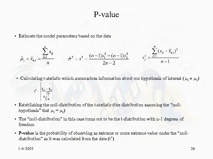
P-value • Estimate the model parameters based on the data • Calculating t-statistic which summarizes information about our hypothesis of interest ( 1 2) • Establishing the null-distribution of the t-statistic (the distribution assuming the “nullhypothesis” that 1 = 2) • The “null-distribution” in this case turns out to be the t-distribution with n-1 degrees of freedom • P-value is the probability of observing as extreme or more extreme value under the “nulldistribution” as it was calculated from the data (t*) 1 -4 -2005 26
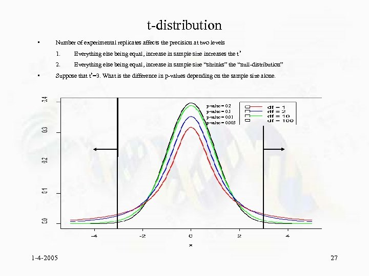
t-distribution • Number of experimental replicates affects the precision at two levels 1. 2. • Everything else being equal, increase in sample size increases the t * Everything else being equal, increase in sample size “shrinks” the “null-distribution” Suppose that t*=3. What is the difference in p-values depending on the sample size alone. p-value = 0. 2 p-value = 0. 1 p-value = 0. 003 1 -4 -2005 27
bf9a08a78a4d802da771364db7e8ae92.ppt