Compressing Texture Coordinates with h Selective Linear Predictions

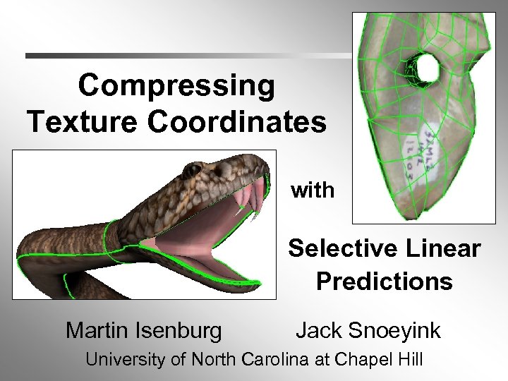Compressing Texture Coordinates with h Selective Linear Predictions Martin Isenburg Jack Snoeyink University of North Carolina at Chapel Hill

Take this home: “We predict texture coordinates with four different rules – taking into account the presence of mapping discontinuities. ” “We compress the corresponding corrective vectors with different arithmetic contexts. ”

Overview • • Background Compressing Vertex Positions Linear Prediction Schemes Texture Coordinate Mappings Compressing Texture Coordinates Alternative Approaches Summary

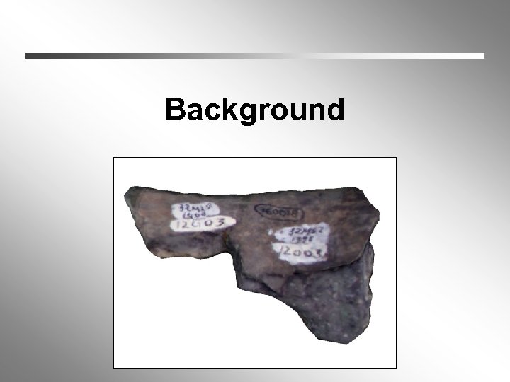Background

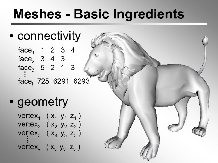Meshes - Basic Ingredients • connectivity face 1 1 2 3 4 face 2 3 4 3 face 3 5 2 1 3 facef 725 6291 6293 • geometry vertex 1 ( x 1 y 1 z 1 ) vertex 2 ( x 2 y 2 z 2 ) vertex 3 ( x 3 y 3 z 3 ) vertexv ( xv yv zv )

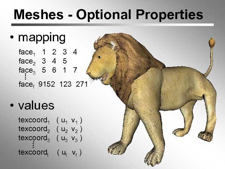Meshes - Optional Properties • mapping face 1 1 2 3 4 face 2 3 4 5 face 3 5 6 1 7 facef 9152 123 271 • values texcoord 1 ( u 1 v 1 ) texcoord 2 ( u 2 v 2 ) texcoord 3 ( u 3 v 3 ) texcoordt ( ut v t )

Mesh Compression • Geometry Compression [Deering, 95] – Fast Rendering – Progressive Transmission – Maximum Compression

Mesh Compression Deering, • Geometry Compression [[Deering, 95] – Fast Rendering – Progressive Transmission – Maximum Compression • • • Connectivity Geometry Properties

Mesh Compression Deering, • Geometry Compression [[Deering, 95] – Fast Rendering – Progressive Transmission – Maximum Compression • • • Connectivity Geometry Properties – Mapping – Values Normals Colors Material Attributes Texture Coordinates

Triangle Mesh Compression [Touma & Gotsman, Graphics Interface 98] • Connectivity “coding with vertex degrees” - optimal? • Geometry “parallelogram prediction” - most popular! • Texture Coordinates ? ? ? “… treat like vertex positions …” Yes! But …

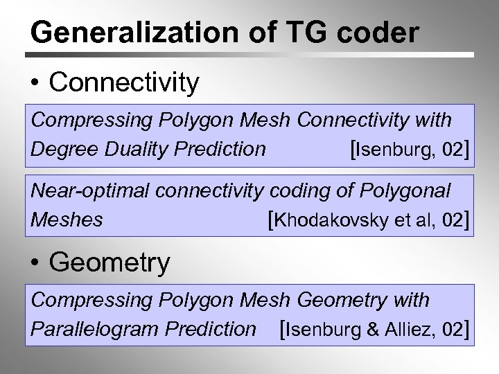Generalization of TG coder • Connectivity Compressing Polygon Mesh Connectivity with Degree Duality Prediction [Isenburg, 02] Near-optimal connectivity coding of Polygonal Meshes [Khodakovsky et al, 02] • Geometry Compressing Polygon Mesh Geometry with Parallelogram Prediction [Isenburg & Alliez, 02]

Compressing Vertex Positions

Compressing Vertex Positions • Classic approaches [95 – 98]: – linear prediction Geometry Compression Java 3 D [Deering, 95] Geometric Compression through topological surgery [Taubin & Rossignac, 98] MPEG - 4 Triangle Mesh Compression Virtue 3 D [Touma & Gotsman, 98]

Compressing Vertex Positions • Classic approaches [95 – 98]: – linear prediction • Recent approaches [00 – 02]: – – – spectral re-meshing space-dividing vector-quantization feature discovery angle-based

Compressing Vertex Positions • Classic approaches [95 – 98]: – linear prediction • Recent approaches [00 – 02]: – – – spectral Spectral Compression of Mesh Geometry re-meshing [Karni & Gotsman, 00] space-dividing vector-quantization feature discovery expensive numerical computations angle-based

Compressing Vertex Positions • Classic approaches [95 – 98]: – linear prediction • Recent approaches [00 – 02]: – – – spectral Progressive Geometry Compression re-meshing [Khodakovsky et al. , 00] space-dividing vector-quantization feature discovery modifies mesh prior to compression angle-based

Compressing Vertex Positions • Classic approaches [95 – 98]: – linear prediction • Recent approaches [00 – 02]: – – – spectral Geometric Compression for interactive transmission re-meshing [Devillers & Gandoin, 00] space-dividing vector-quantization feature discovery poly-soups; complex geometric algorithms angle-based

Compressing Vertex Positions • Classic approaches [95 – 98]: – linear prediction • Recent approaches [00 – 02]: – – – spectral Vertex data compression for triangle meshes re-meshing [Lee & Ko, 00] space-dividing vector-quantization feature discovery local coord-system + vector-quantization angle-based

Compressing Vertex Positions • Classic approaches [95 – 98]: – linear prediction • Recent approaches [00 – 02]: – – – spectral Compression of engineering models by repeated feature re-meshing discovery [Shikhare et al. , 01] space-dividing vector-quantization feature discovery certain 3 D models + expensive matching angle-based

Compressing Vertex Positions • Classic approaches [95 – 98]: – linear prediction • Recent approaches [00 – 02]: – – – spectral Angle-Analyzer: A trianglequad mesh codec re-meshing [Lee, Alliez & Desbrun, 02] space-dividing vector-quantization feature discovery dihedral + internal = heavy trigonometry angle-based

Linear Prediction Schemes

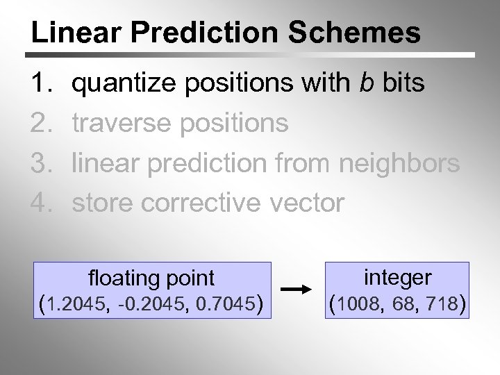Linear Prediction Schemes 1. 2. 3. 4. quantize positions with b bits traverse positions linear prediction from neighbors store corrective vector floating point (1. 2045, -0. 2045, 0. 7045) integer (1008, 68, 718)

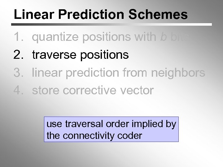Linear Prediction Schemes 1. 2. 3. 4. quantize positions with b bits traverse positions linear prediction from neighbors store corrective vector use traversal order implied by the connectivity coder

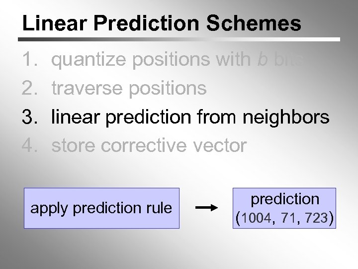Linear Prediction Schemes 1. 2. 3. 4. quantize positions with b bits traverse positions linear prediction from neighbors store corrective vector apply prediction rule prediction (1004, 71, 723)

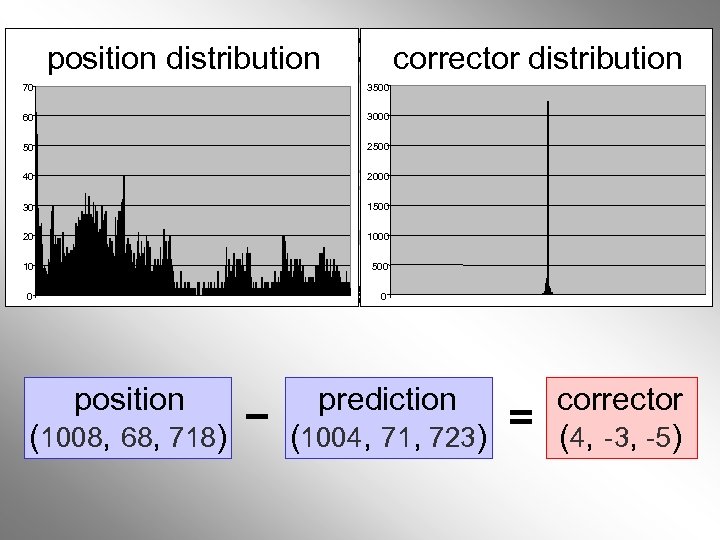Linear Prediction Schemes position distribution corrector distribution 3500 70 60 50 40 30 20 10 0 1. 2. 3. 4. quantize positions with b bits traverse positions linear prediction from neighbors store corrective vector position (1008, 68, 718) 3000 2500 2000 1500 1000 500 0 prediction (1004, 71, 723) corrector (4, -3, -5)

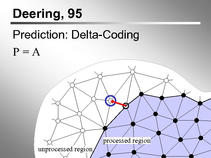Deering, 95 Prediction: Delta-Coding P=A P A processed region unprocessed region

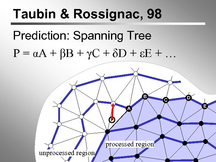Taubin & Rossignac, 98 Prediction: Spanning Tree P = αA + βB + γC + δD + εE + … B A P processed region unprocessed region C D E

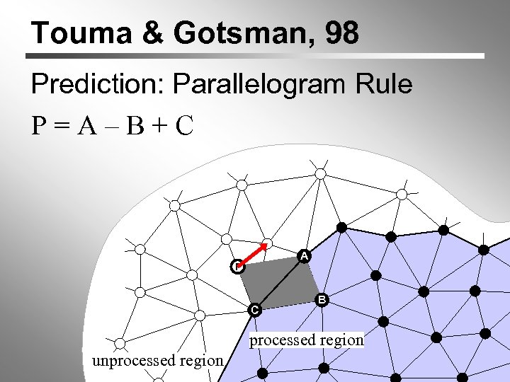Touma & Gotsman, 98 Prediction: Parallelogram Rule P=A–B+C A P C B processed region unprocessed region

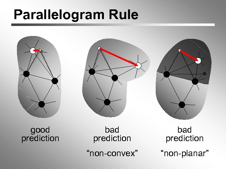Parallelogram Rule good prediction bad prediction “non-convex” “non-planar”

Not Triangles … Polygons! Face Fixer [Isenburg & Snoeyink, 00]

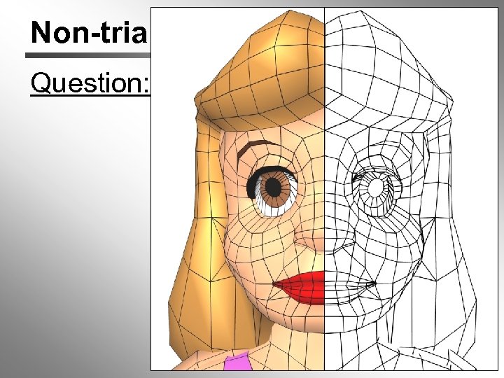Non-triangular Faces Question: Why would a mesh have a non-triangular face?

Non-triangular Faces Question: Answer: Why would a mesh have a non-triangular face? Because there was no reason to triangulate it! This face was “convex” and “planar”. use this info for better predictions

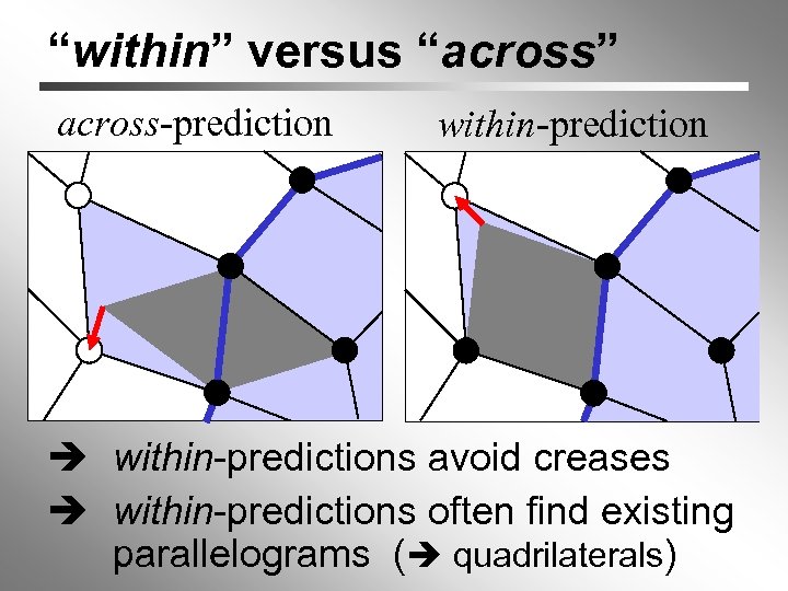“within” versus “across” across-prediction within-predictions avoid creases within-predictions often find existing parallelograms ( quadrilaterals)

Texture Coordinate Mappings

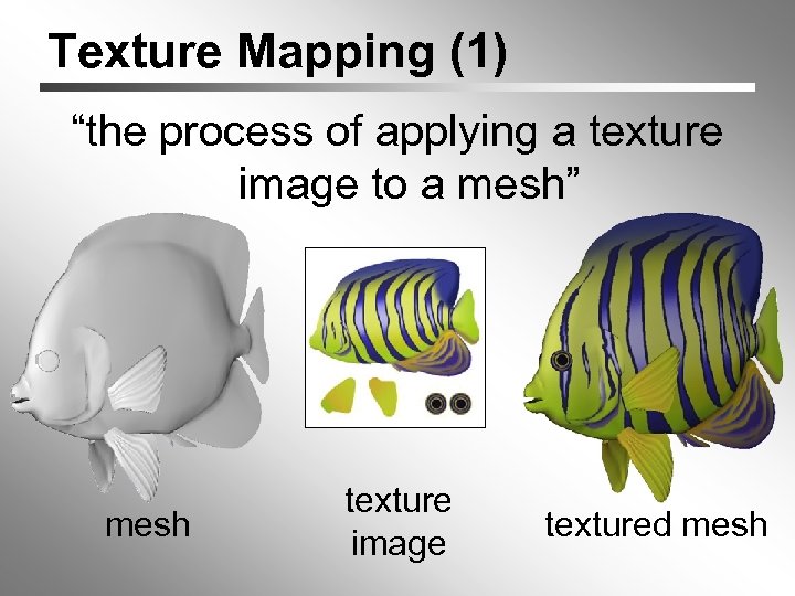Texture Mapping (1) “the process of applying a texture image to a mesh” mesh texture image textured mesh

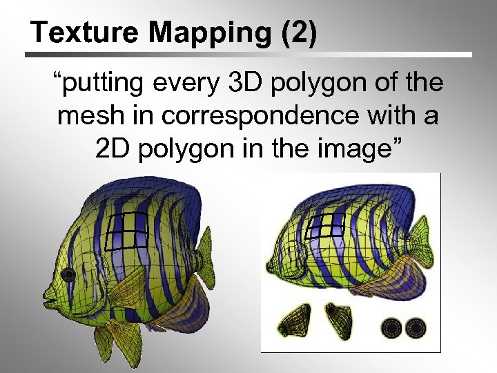Texture Mapping (2) “putting every 3 D polygon of the mesh in correspondence with a 2 D polygon in the image”

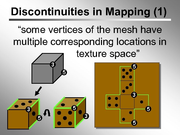Discontinuities in Mapping (1) “some vertices of the mesh have multiple corresponding locations in texture space” 3 5 5 3 5

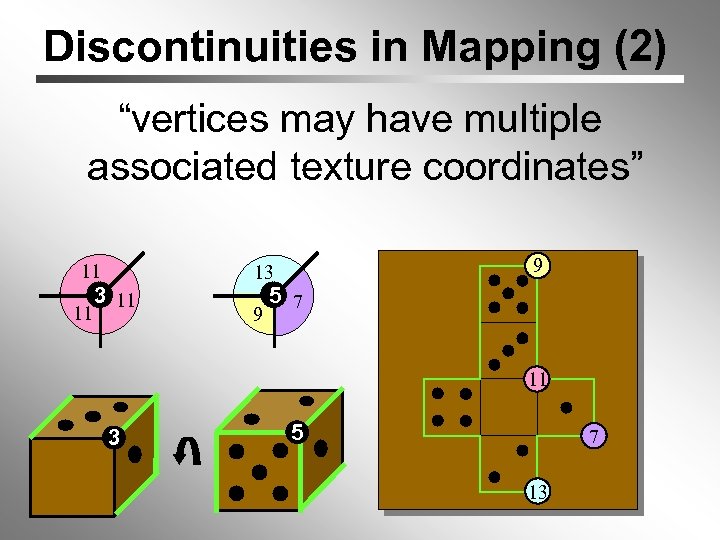Discontinuities in Mapping (2) “vertices may have multiple associated texture coordinates” 11 11 3 11 9 13 9 5 7 11 3 5 7 13

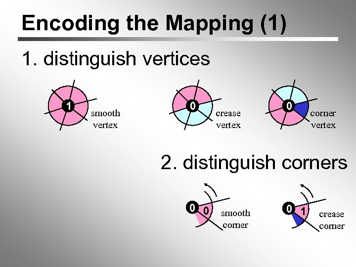Encoding the Mapping (1) 1. distinguish vertices 1 smooth vertex 0 crease vertex 0 corner vertex 2. distinguish corners 0 0 smooth corner 0 1 crease corner

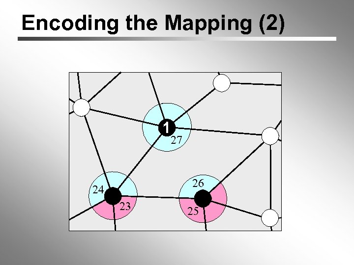Encoding the Mapping (2) 1 27 26 24 23 25

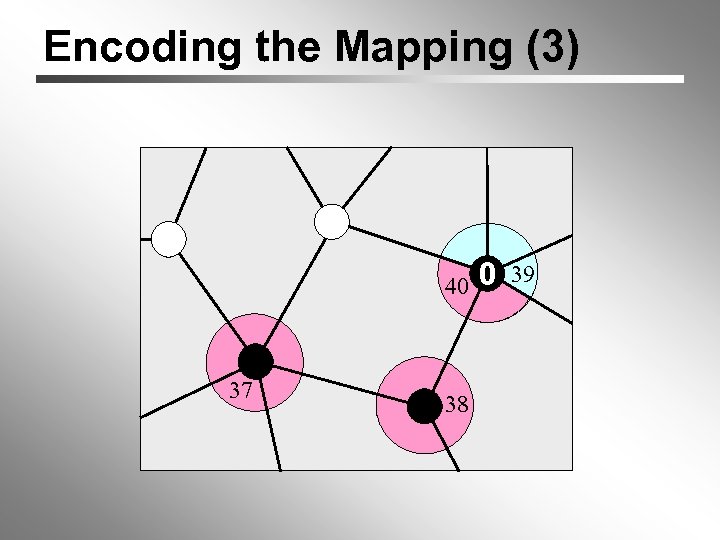Encoding the Mapping (3) 0 0 1 40 0 39 1 0 37 38

Why Discontinuities ? • cuts required to flatten mesh – no boundary – non-zero genus • piece-wise texture mapping – author / artist decision – easier for automated techniques • additional cuts to meet objectives – angle/area preserving parameterization – minimizing texture stretch

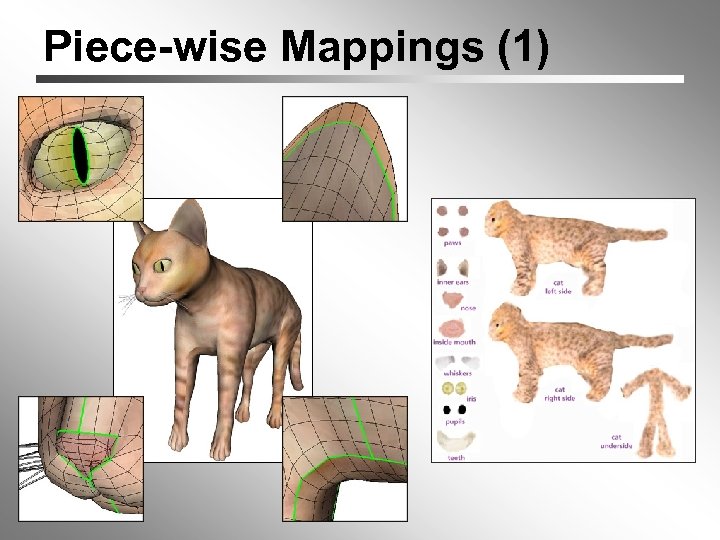Piece-wise Mappings (1)

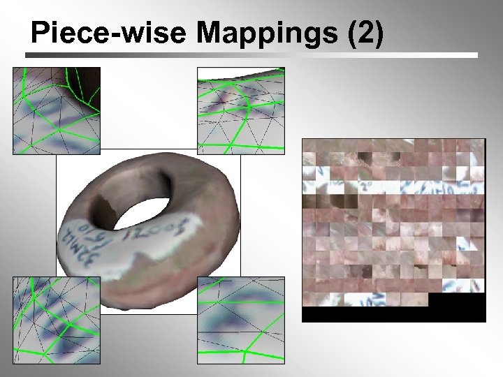Piece-wise Mappings (2)

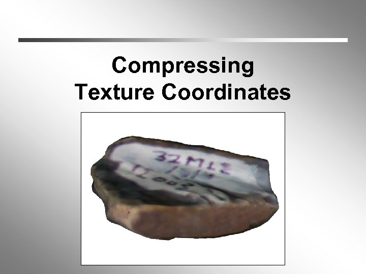Compressing Texture Coordinates

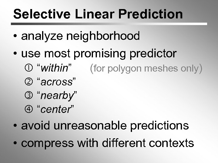Selective Linear Prediction • analyze neighborhood • use most promising predictor “within” “across” “nearby” “center” (for polygon meshes only) • avoid unreasonable predictions • compress with different contexts

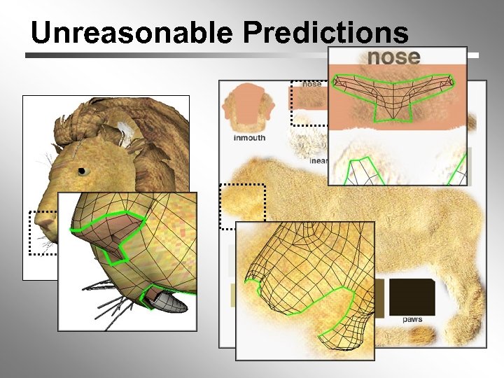Unreasonable Predictions

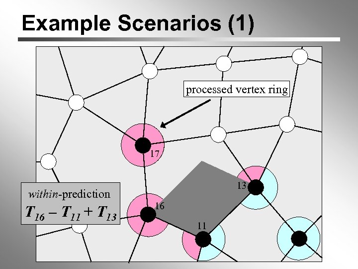Example Scenarios (1) processed vertex ring 1 17 13 within-prediction T 16 – T 11 + T 13 16 11

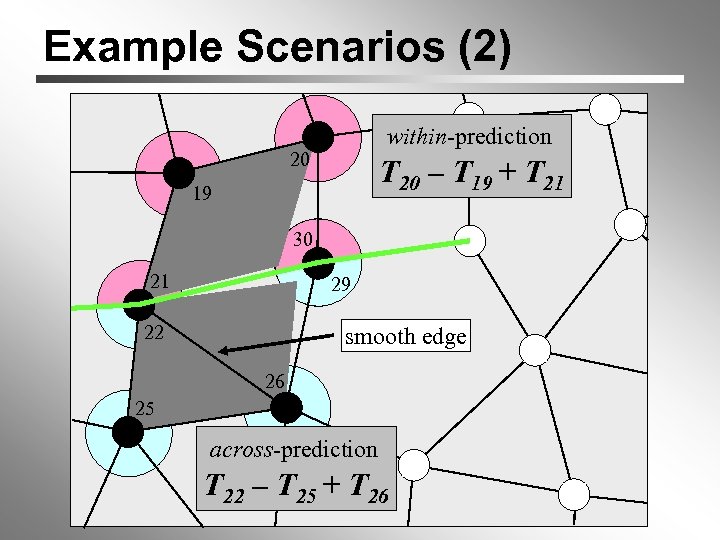Example Scenarios (2) within-prediction 20 T 20 – T 19 + T 21 19 30 0 1 21 1 22 0 29 0 smooth edge 26 25 across-prediction T 22 – T 25 + T 26

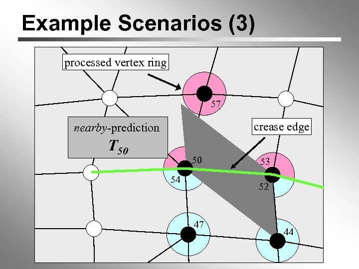Example Scenarios (3) processed vertex ring 1 57 crease edge nearby-prediction T 50 50 54 53 52 47 44

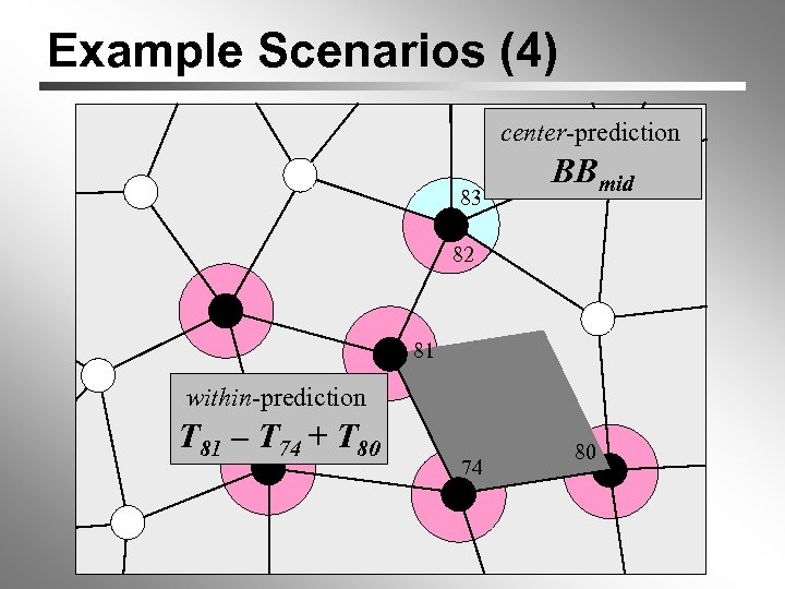Example Scenarios (4) center-prediction 0 0 83 1 0 1 82 0 BBmid 81 within-prediction T 81 – T 74 + T 80 74 80

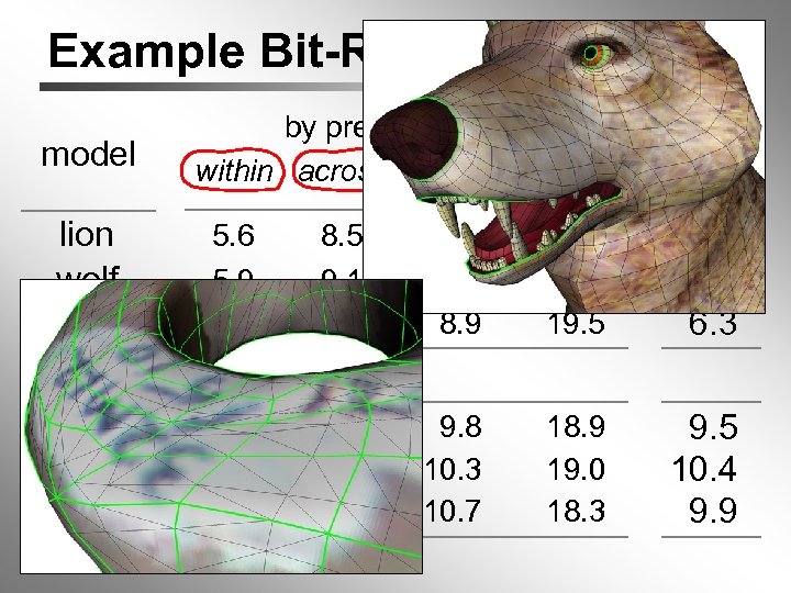Example Bit-Rates (10 bit) model by prediction type within across nearby center total lion wolf raptor 5. 6 5. 9 5. 5 8. 5 9. 1 8. 4 9. 7 11. 1 8. 9 20. 2 19. 5 6. 3 6. 6 6. 3 “ 1398” “ 1412” “ 1510” -. - 7. 5 8. 3 7. 3 9. 8 10. 3 10. 7 18. 9 19. 0 18. 3 9. 5 10. 4 9. 9

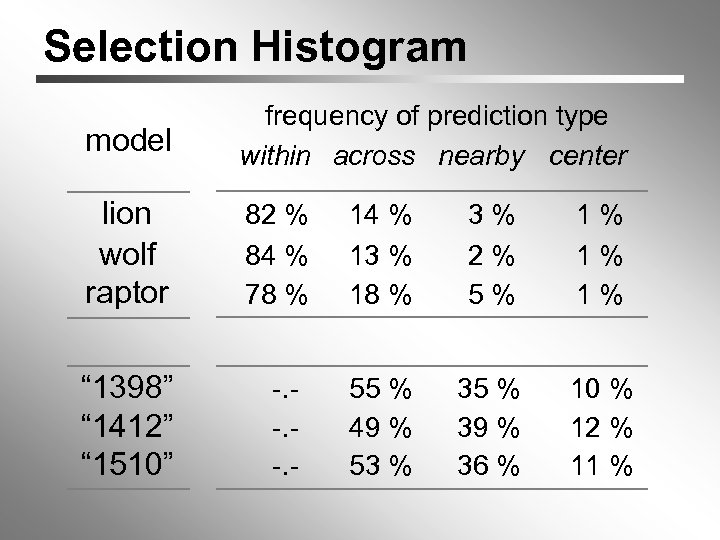Selection Histogram model frequency of prediction type within across nearby center lion wolf raptor 82 % 84 % 78 % “ 1398” “ 1412” “ 1510” -. - 14 % 13 % 18 % 3% 2% 5% 1% 1% 1% 55 % 49 % 53 % 35 % 39 % 36 % 10 % 12 % 11 %

Alternative Approaches

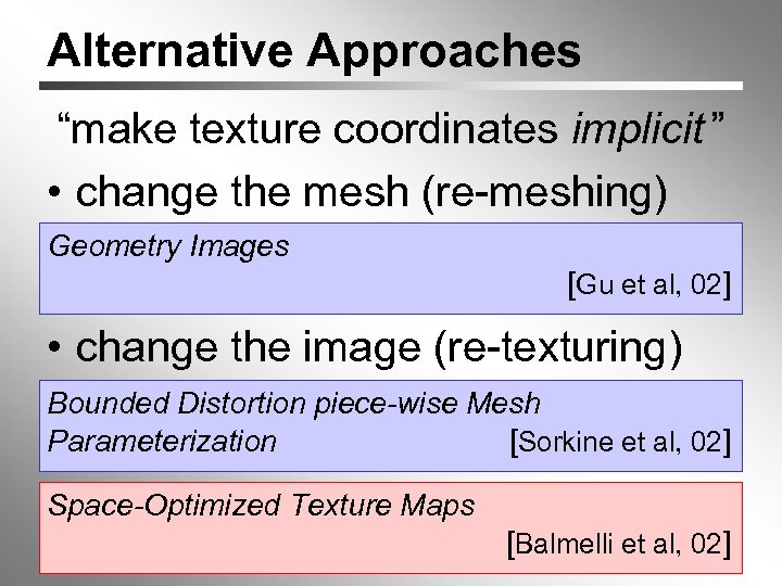Alternative Approaches “make texture coordinates implicit ” • change the mesh (re-meshing) Geometry Images [Gu et al, 02] • change the image (re-texturing) Bounded Distortion piece-wise Mesh Parameterization [Sorkine et al, 02] Space-Optimized Texture Maps [Balmelli et al, 02]

Summary & Acknowledgments

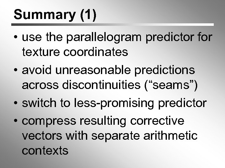Summary (1) • use the parallelogram predictor for texture coordinates • avoid unreasonable predictions across discontinuities (“seams”) • switch to less-promising predictor • compress resulting corrective vectors with separate arithmetic contexts

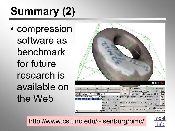Summary (2) • compression software as benchmark for future research is available on the Web http: //www. cs. unc. edu/~isenburg/pmc/ local link

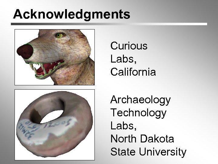Acknowledgments Curious Labs, California Archaeology Technology Labs, North Dakota State University

Thank You! http: //www. cs. unc. edu/~isenburg/pmc/